Translate this page into:
Dynamical approach in studying stability condition of exponential (GARCH) models
⁎Corresponding author. gabbarfalcon@st.tu.edu.iq (Abduljabbar Ali Mudhir)
-
Received: ,
Accepted: ,
This article was originally published by Elsevier and was migrated to Scientific Scholar after the change of Publisher.
Peer review under responsibility of King Saud University.
Abstract
In this article our goal is to studying the stationary condition of EGARCH time series model which is proved by Nelson (1991) but what we did is to prove it with more simple and clearly defined method and this is done by using a dynamical approximation relying on local linearization method in the neighborhood of a non-zero singular point of EGARCH model. This method is being used to approximate a Nonlinear model to a linear autoregressive model. Beside that we found the orbitally stability condition of a limit cycle of EGARCH(1,1) model if the model possess it.
Keywords
EGARCH
Local linearization method
Conditional variance
Limit cycle
Time series
Autoregressive model

1 Introduction
The exponential generalized autoregressive conditional heteroskedastic time series model denoted by (EGARCH) model is an extension for (GARCH) model proposed by Nelson in 1991. The model came from ARCH family models which are proposed to deal with the volatility in time series data (Francq and Zakoian, 2010) which known later the conditional heteroskedastic in variance or in another words the variance depends on time and changes over time (t) namely conditional variance ( ), these models are made the conditional variance as a function of time (Nelson 1991).
The stationarity of any stochastic process requires that the variance must be constant and independent of time (t). So we will use a dynamical approaches based on a local linearization technique near the non-zero singular point of EGARCH model to approximate this model to a linear model in the neighborhood of the non-zero singular point, this method play a major rule in convergence of conditional variance to an unconditional variance which is constant and independent of time as t approach to infinite.
In a non-linear time series models the stochastic difference equation known as: where is nonlinear function and , i.e. is a white noise process, and in GARCH models the stochastic difference equation became: where . The clear motivation is under what conditions the conditional variance converges to unconditional variance . This is what we will discuss in the article.
We must refer to that many researchers use a local linearization technique in finding a stability conditions for many non-linear autoregressive models, Ozaki in 1985 used this method to find a stability condition of EXPAR(P) model, Mohammad and Salim in 2007 used it for the logistic LSTAR(P) model, Mohammed and Ghannam in 2010 used it for the Cauchy model, Salim and Younis studied this method in 2012, also Mohammad and Ghaffar in 2016 used it for the GARCH model (Mohammad and Ghaffar, 2016; Mohammad and Ghannam, 2010; Mohammad and Salim, 2007; Ozaki, 1985; Salim and Youns, 2012).
The methodological development in this paper is to prove the stationary condition of the EGARCH model by using local linearization method which looks simpler and clearly defined.
2 Preliminaries
The purpose of this section is to introduce some basic concepts and definitions to get a fully understanding for the study.
Definition 2.1 Singular point and it's stability (Ozaki 1985; Salim and Youns, 2012)
A point
is a singular point of a function
if satisfies:
and for the model:
Definition 2.2 Limit cycle and it's stability (Ozaki 1985; Salim and Youns 2012)
A limit cycle of the model (2.1) is defined as an isolated and closed trajectory of the form: such that is a positive integer. The word ''closed'' means that if the initial value belongs to the limit cycle, then: the word ''isolated'' means that every trajectory beginning sufficiently near the limit cycle approaches it either for .
If it approaches the limit cycle for we call it a ''stable limit cycle'', and if it approaches the limit cycle for we call it an ''unstable limit cycle''. The smallest integer which satisfies this definition is called the period of the limit cycle of the model (2.1).
Definition 2.3 Autoregressive model of general order (Priestely, 1981)
A linear Autoregressive model of order denoted by AR( ) has the form: by using a Backward shift operator the AR( ) model can be written in: the general solution of the model is given by: such that is the complementary function which is the solution of homogenous difference equation: and in general will has the form: where is an arbitrary constants and is the roots of the polynomial the autoregressive model AR( ) is an asymptotically stationary process if:
which implies that all the roots of must lie inside the unit circle,
Background of the model
The Exponential Generalized Autoregressive Conditional Heteroskedasticity (EGARCH) models descend from ''ARCH models'' family which is created by Robert Engle in 1982 (Engle, 1982) as one of the nonlinear time series models. ARCH models can be expressed as the following form:
After four years later in Bollerslev (1986) extended the study of ARCH models and proposed the Generalized Autoregressive Conditional Heteroskedasticity models [GARCH(Q,P)] which can expressed as:
This model is being used in many studies and a family of models emerged from it as an extension of GARCH models like GJR-GARCH model by Glosten, Jagannathan and Runkle. TARCH model introduced by Zakoian in 1994. PARCH model by Ding et al. in 1993….etc. It has a great importance because it is modeling the volatility in data that exists in several stochastic processes such as financial time series. One of its most important properties; is that GARCH models can capture thick tailed returns and volatility clustering, nevertheless GARCH model has three drawbacks (Nelson, 1991): Firstly, it fails to capture ''leverage effect'' that was mentioned by Black in 1976 when he described it by saying: ''stock returns are negatively correlated to changes in returns volatility implying that volatility tends to rise in response to bad news and fall in response to good news'' (Black, 1976). Secondly, is that GARCH model depends only on the magnitude of the changing in series data. Thirdly, there is a positivity constraint on its parameters clearly in model's formula. Because of that Daniel B. Nelson (Nelson, 1991) introduced the EGARCH model which can avoid these shortcomings so that EGARCH model consists a term of the leverage effect and that is noticed in its formula what make the model become depending on the magnitude and sign of the changing in series data. Also the existence of the logarithm in the formula of the model cancels the positivity constraints on its parameters (Bollerslev et al., 1994).
The EGARCH model has got a big attention and many researchers used EGARCH to modeling data like stock prices, gold and oil prices, exchange rates … etc.
Definition 2.4 EGARCH(Q,P) Process (Francq and Zakoian, 2010)
Let
be an identical independent distributed sequence such that:
Then
is said to be an Exponential Generalized Autoregressive Conditional Heteroskedasticity process can be expressed as [EGARCH(Q,P)] if it satisfies an equation of the form:
To explain the magnitude and the sign mentioned above through the formula of the model. The terms and represent the magnitude and the sign effect respectively. Also the leverage effect is represented in the term , the ARCH effect is represented in and is the GARCH effect term.
The function in (2.3) is a function of both of magnitude and sign, this allows to the EGARCH process to response to the rises and the falls of the series data especially in the financial time series data. Therefore EGARCH models classified under what known later as asymmetric models which are defined the asymmetric relation between returns and the change in volatility (Bollerslev et al., 1994).
3 Stationary condition of EGARCH(Q,P) process
Theorem 3.1 Francq and Zakoian, 2010
Assume that is not almost surely equal to zero and that the polynomials have no common root with not identically null then the EGARCH(Q,P) model admit a strictly stationary iff the roots of are outside the unit circle.
The stationary condition in the above theorm is same as the stationary condition of a general autoregressive process exactly with finite innovation variance.
Our contribution in this paper is to find the stationary condition mentioned in Theorem 2.1 and prove it by using dynamical approach. In order to showing that we need the following lemma:
Lemma 3.1 Mohammad and Ghaffar, 2016
Let
be a non-negative real numbers. The following polynomial:
does not have a roots inside and on the unit circle if and only if .
Let be and let are non-negative real numbers.
Thus: this implies: so that: then by hypothesis we obtain: this means the polynomial (3.1) has no any roots inside and on the unit circle since all the roots that lie between 0 and 1 doesn't verify .
Conversely; suppose that polynomial 3.1 doesn't have any roots inside the unit circle, so that is one of the roots of polynomial 3.1, and then: and since , then and since h is one of the roots then , so that . □
Now, consider the general form of the EGARCH(Q,P):
To find the stability condition of EGARCH(Q,P) model in term of its parameters by using a dynamical approach. First, we should find the non-zero singular point of the model which is corresponding to unconditional variance .
By taking the mathematical expectation of both sides of (3.2) we get:
As
we notice that:
So we obtain:
The non-zero singular point for EGARCH(Q,P) model is stable if:
Let be the non-zero singular point of EGARCH(Q,P). near the non-zero singular or in the neighborhood of with sufficiently small radius such that: and by using the variational equation: and by substitute this equation in (3.3) we get: From (3.3) and by using expansion of and since , we get: multiply both sides by as a constant, we obtain: this is a linear difference equation of order Q. If we can put the polynomial by using lag operator in the form: then the stability requires that the all roots of the polynomial: lie outside the unit circle which is by lemma (1) corresponding to the condition . □
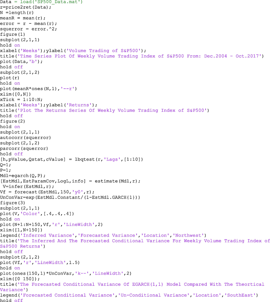
By using Matlab (R2016a) software for modeling weekly volume trading S&P500 index from Dec. 2004–Oct. 2017 downloaded from yahoo finance website with 670 observation in EGARCH(1,1) model we notice the general form of the series data and the return series in the following figure (Fig. 1):We can check for the heteroskedasticity from the autocorrelation and partial autocorrelation function plot of the squared return errors of the series data also we used Ljung–Box Q-test to check the heteroskedasticity (Fig. 2).
After fitting the data with EGARCH(1,1) model we can see in Fig. 3 that the forecasted conditional variance converge to the unconditional variance which is corresponding with the non-zero singular point value as in Eq. (3.4).
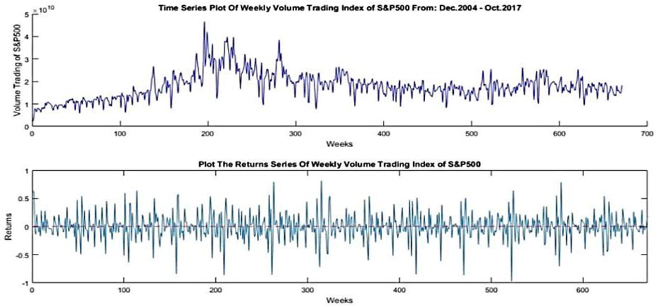
- The general form of the series data and the return series.
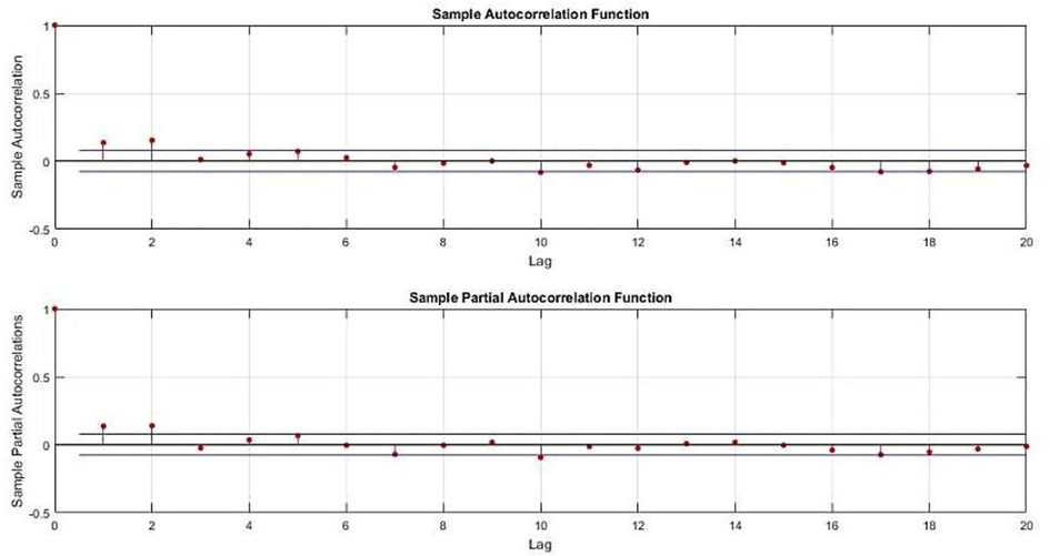
- The autocorrelation and partial autocorrelation function plot of the squared return errors of the series data.
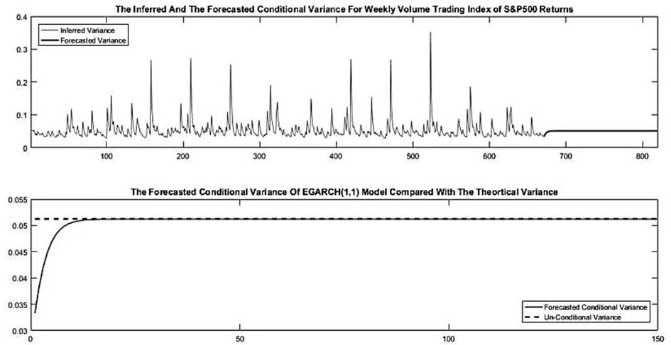
- The forecasted conditional variance converge to the unconditional variance.
4 The orbitally stability of the limit cycle
To study and find a stability conditions of the limit cycle for the EGARCH(Q,P) model if it exists, we begin to find the stability condition for the EGARCH(1,1).
The limit cycle with period of EGARCH(1,1) is orbitally stable if the following condition satisfied:
Suppose that the model possess a limit cycle of period
namely:
near the neighborhood of each point of this limit cycle, let
be the radius of the neighborhood sufficiently small such that:
by using the assignment equation
we substitute this equation in the model EGARCH(1,1) which is can get it by putting Q = P=1 in Eq. (3.2) and taking the mathematical expectation:
Now, by iterate Eq. (4.2) for times we get: equivantely: and hence the limit cycle is orbitally stable if: or in another form:
5 Conclusion
The study summarizes in knowing whether it adds an interest to the statistical literature, it introduces another method in proving the stationary condition of EGARCH model. This method was applied in some models previously by a group of researchers in 2007 until 2016 based on the manner of Ozaki and Tong in 1985 and 1990 respectively.
The Autoregressive Conditional Heteroskedasticity models have conditional variance changing over time and this is a problematic for prediction. This method approximate the nonlinear model to linear model near its singular point and as a result will fix the conditional variance to unconditional variance which its value is equal to the value of the non-zero singular point and then these models mix with linear models to get a composite models for forecast in future.
In Section 3 we use local linearization method to prove the stability condition of the model EGARCH(Q,P) in terms of its parameters, this condition help us to know whether the non-zero singular point is stable or not.
In Section 4 we gave a stability condition of the limit cycle in case that the model possesses it. In fact, if the process doesn't have any stable singular point then it doesn't necessary mean that the process goes to have stable limit cycle, it can be a model doesn't have any stable singular point nor stable limit cycle.
References
- Black, Fischer, 1976. Studies of Stock Price Volatility Changes. In: Proceedings of the 1976 Meeting of the Business and Economic Statistics Section. American Statistical Association, Washington DC, 177–181.
- Generalized Autoregressive Conditional Heteroskedasticity. J. Econ.. 1986;31:307-327.
- [Google Scholar]
- Arch Models. In: Bollerslev Tim, Engle Robert F., Nelson Daniel B., eds. Handbook of Econometrics. Vol 4. 1994. p. :2961-3031. (Chapter 49)
- [Google Scholar]
- Autoregressive conditional heteroscedasticity with estimate of the variance of United Kingdom Inflation. Econometrica – The Econometric Soc.. 1982;50(4):987-1007.
- [Google Scholar]
- GARCH Models (first ed.). John Wiley & Sons Ltd; 2010.
- Studying the stability of conditional variances for GARCH models with application. Tikrit University J. Pure Sci.. 2016;1662:271-280.
- [Google Scholar]
- Stability of Cauchy autoregressive model. Zanco, J. Pure Appl. Sci. – Sallahaddin University – Hawler 2010 (special Issue)
- [Google Scholar]
- Conditional Heteroskedasticity in Asset Returns: a new approach. Econometrica – The Econometric Soc.. 1991;59(2):347-370.
- [Google Scholar]
- Non-Linear Time Series Models and Dynamical Systems. Elsevier Science Publishers. 1985;5(2):25-83.
- [Google Scholar]
- Spectral Analysis and Time Series. London: Academic Press INC; 1981. p. :1.
- A Study of the Stability of a Non-Linear Autoregressive Models. Australian J. Basic Appl. Sci.. 2012;6(13):159-166.
- [Google Scholar]
- Nonlinear Time Series A Dynamical System Approach. New York: Oxford University Press; 1990.
Appendix: Matlab modeling program for Example 3.1