

Translate this page into:
Direct Solution of Using Three Point Block Method of Order Eight with Applications
⁎Corresponding author. rlogmany@outlook.com (Reem Allogmany)
-
Received: ,
Accepted: ,
This article was originally published by Elsevier and was migrated to Scientific Scholar after the change of Publisher.
Abstract
This study aims to construct an implicit block method with three-point to tackle general second-order ordinary differential equations (ODEs) directly. Hermite Interpolating Polynomial is used as the fundamental function to obtain the proposed method which involved the first and second derivatives of . From the investigation done, it was found that the proposed method is consistent and zero-stable, hence it is convergent. The proposed method’s efficiency was obtained and a comparison was made in terms of accuracy to some existing methods with similar order or higher than it. This new method is able to solve linear and nonlinear initial value problems of the general second-order ODEs and outperformed existing methods with impressive results. Applications of the new method such as in the Fermi-Pasta-Ulam problem and van der Pol oscillator are discussed.
Keywords
Block
Second-order
IVPs
Hermite interpolation
Implicit

1 Introduction
Many problems in applied science, physics, chemistry, and engineering are modeled as second-order ordinary differential equations (ODEs) (Boatto et al., 1993; Troy, 1993). For instance, orbital dynamics problems, electric circuit, damped and undamped spring-mass or any problem including Newton second law of motion. A good number of literature is available for the solutions of second-order ODEs, especially the special case (Mansor et al., 2017; Liu et al., 2019; Mehdizadeh and Shokri, 2020). Other methods, among others that attempted to integrate general second-order ODEs directly, are due to Waeleh and Majid (2017), Abdelrahim et al. (2016), Omar et al. (2017), Nasir et al. (2018), Singh and Ramos (2019) and Hashim et al. (2019) etc. Moreover, recently, several studies have been conducted to implement derivative methods in solving ODEs, but these methods have only the first derivative of
, (see Cash, 1981; Ismail and Ibrahim, 1999; Hojjati et al., 2006; Khalsaraei et al., 2012; Mohamed et al., 2018; Ramos and Rufai, 2019; Turki et al., 2020; Lee et al., 2020), which revealed that adding more derivatives might lead to more accurate numerical schemes. Meanwhile, block methods have been utilized to produce
-point of the approximate solutions at a step simultaneously. Each block contains
-point approximation values of
, at each iteration. The block method is first presented by Milne and Milne (1953) which is later extended by many scholars, (Badmus, 2014; Allogmany et al., 2019; Adeyeye and Omar, 2019; Allogmany et al., 2020; Allogmany and Ismail, 2020). In recent literature, hybrid numerical approaches have been developed with more function evaluations to obtain approximate solutions with very high precision, (see Jator, 2010; Badmus, 2014; Adeyeye and Omar, 2017; Singh and Ramos, 2019; Adeyeye and Omar, 2019). In general, A direct solution can be provided by using interpolation and collocation technique, (Awoyemi et al., 2011; Kuboye and Omar, 2015; Ramos and Rufai, 2018; Obarhua and Kayode, 2020). However, to determine the coefficients of the method via collocation and interpolation approach, the points must be collocated and interpolated these results in a system of linear equations which have to be solved simultaneously. Therefore, in this study, our main concern is to come up with a direct three-point block implicit method with extra derivatives by using a strategy which can be easily executed for directly solving both linear and nonlinear problems in the form of
Let us supposed that the higher derivatives of f in (1) exist and meet the requirement of the Lipschitz condition as below:
. Then, the IVPs in (1) has a unique solution in R (see Wend, 1969; Wend, 1967).
The method is able to approximate solution of (1) at three points simultaneously using interpolation and integration procedure, which involved the first and second derivatives of with constant step-size. Where these derivatives are
The paper is structured as follows: In Section 2, the derivation of the three-point implicit block method of order eight (DI3PB) is presented. Section 3, analysis of the main properties of the proposed method including order, stability, consistency, and convergence, is presented. Section 4 is dedicated for implementation procedure the method. The outcome of the numerical experiment of the method is given in Section 5. Lastly, Section 6 provided the study’s conclusion.
2 Derivation of Method
In the three-point block method, the interval
is divided into a series of blocks that generate three approximate values,
and
, at each block, concurrently using one earlier block. In Fig. 1, the idea is illustrated where
is the first point and
is the last point of the block with step size
where h is constant step-size,
and
.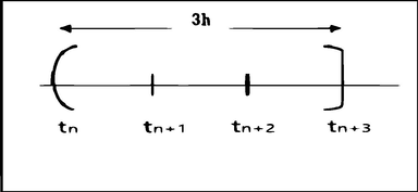
Three point block.
The derivation of the method is done by integrating Eq. (1) to come up with the approximate solution and .
Integrating the first, second, and the third point once gives:
Integrating twice gives:
In order to estimate
in Eq. (1), we will use the Polynomial of Hermite interpolating
(Stoer and Bulirsch, 1991). The polynomial has the following form
is the generalized Lagrange polynomial, and .
For the first point,
, let
and
be substituted into (5). By calculating the integral from
to
. MAPLE was used to carry out the computations
Where g and q denote the third and fourth derivatives of the solution, respectively.
Applying similar technique by taking
and
for the second point,
, and calculating the integral from
to
. MAPLE was used to carry out the computations
For the third point, we take
and
. similarly, we calculate the integral from
to 0. MAPLE was used to carry out the computations
3 Properties of the method
3.1 Order of the method
To verify the order of the proposed method, we write Eqs. (9)–(14) in the matrix difference equation as below:
Where , and are matrices of coefficients defined as
We assume
is a sufficiently differentiable function. Next, we write the difference operator L associated with the implicit block method (9)-(14) as
By applying (17) in the new method we have that and .
Hence, we conclude that the proposed method DI3PB is of order , and is the error constant. As the order of the proposed method is , then, the proposed method is consistent (Lambert, 1991).
3.2 Zero-stability
To check the zero-stability of the direct three-point block method, we rewrite Eqs. (9)–(14) as
identity matrix,
Following Lambert (1973), a method is said to be zero-stable if the roots of the first characteristic polynomial satisfies .
Then, implies that , as a result, .
Thus, the method is zero stable. The direct three-point implicit block method (9)-(14) is convergent since it is consistent and zero-stable. (Ackleh et al., 2009).
3.3 Linear Stability
For the linear stability, we substitute the linear test equation
into the formulae of the proposed method. This formulae can be stated in the matrix form as
where
and A,B,C,D,E,F are matrices of
. By setting
and
, the stability polynomial is given as
Where
are matrices of
. Then, we solved (18) for
and
by setting
and
which gives
. The absolute stability region of the method is the shaded region as shown in Fig. 2. Actually, the region is unbounded to the left for
, and
is bounded by 0 and
. Thus, the region almost covers all the lower half plane up to
. It is clear from this figure that the new method has a wider range of stability region compared to the existing methods, (see Waeleh and Majid, 2017; Singh and Ramos, 2019; Kuboye and Omar, 2015). This means we can expect that the new implicit method will cope with IVP better than the existing methods.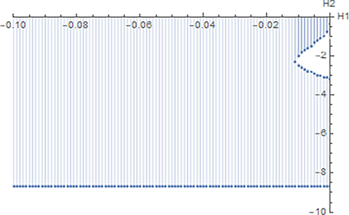
The region of stability for the proposed method.
4 Implementation
The proposed method has been implemented by using the predictor–corrector technique to estimate the approximate solutions of
and
. To compute the starting values, we begin the process by taking Taylor method as the predictor equation:
Then, we evaluate the functions
and
which will be utilize to estimate the solution at the second point as follows
Similarly, we evaluate the functions
and
which will be utilize to estimate the solution at the third point as follows
Next, we evaluate the functions and that we will be used in the next corrector iteration. Then, the next corrector iterations are performed by repeating the procedure given in Eqs. (20)–(22) until the end of the interval.
5 Numerical results
This section assesses the efficiency and accuracy of the proposed DI3PB method with several direct block methods. Here, some well-known test problems alongside the applications problem of Fermi-Pasta-Ulam and van der Pol oscillator are solved by using the proposed 3-point block method. Based on the method, C++ programming codes are developed and applied. Results obtained from the new DI3PB method are compared with those of existing methods with similar or higher order.
Problem 1:
Exact solution:
Problem 2:
Exact solution:
In Problem 1 and Problem 2, we have examined the maximum absolute errors in the given interval using different total steps. In Table 1 and Table 2, the results acquired by the proposed method (DI3PB) are compared with direct 4-point block methods (DFPB) of order five by Abdelrahim et al. (2016) with regards to precision and the total number of steps
, and (FPMBM) of order nine by Waeleh and Majid (2017) with the same number of steps. It is investigated that the results of the proposed method are significantly improved and outperformed both DFPB and FPMBM.
NS
DFPB
NS
FPMBM
DI3PB
1.8627(−9)
5.6512(−12)
1.3207(−16)
2.2223(−15)
1.4247(−16)
5.0902(−16)
6.8052(−17)
1.5108(−15)
6.5156(−16)
1.8765(−15)
2.1578(−16)
NS
DFPB
NS
FPMBM
DI3PB
5.4296(−6)
7.5088(−12)
1.2089(−16)
2.8555(−12)
4.2735(−16)
1.1597(−11)
5.0167(−16)
5.2300(−12)
4.3247(−16)
6.5093(−13)
3.6114(−16)
Problem 3:
Exact solution:
In Problem 3, we calculate the results for different step sizes and check the results found using the new DI3PB method against the variable stepsize hybrid method of order seven (VJAT) in Jator (2010), and the variable stepsize Falkner method of order eight (VFM) in Vigo-Aguiar and Ramos (2006). It is clear from Table 3 that the proposed method yielded better results compared to the existing methods.
NS
VFM
VJAT
DI3PB
7.1122(−07)
6.5286(−11)
7.7716(−16)
9.2632(−08)
1.3679(−11)
1.8874(−15)
1.2108(−10)
1.1897(−12)
1.1601(−15)
Problem 4:
Exact solution:
The numerical results for this problem were obtained using the proposed DI3PB method, the direct hybrid block method of order seven (DHBM) in Adeyeye and Omar (2017), and the direct six-step block method of order seven(DSSB) in Kuboye and Omar (2015), were compared. These three methods satisfy the method of order seven. Accuracy of DI3PB and DHBM are comparable at all step sizes, as presented in Table 4. In addition to that, the numerical result for this proposed method has more accuracy by two decimal places compared to DSSB at
also has more accuracy by five decimal places at
.
h
Method
MAXE
0.01
DI3PB
2.212510(−16)
DHBM
8.881784(−16)
DSSB
1.428607(−11)
0.001
DI3PB
1.526969(−15)
DHBM
2.220446(−15)
DSSB
1.687539(−13)
Problem 5:
Exact solution:
Problem 6:
Exact solution:
We have solved the nonlinear Problem 5 and the linear Problem 6 using the proposed DI3PB method and the existing methods, the direct seven-point hybrid block method (SPH) in Badmus (2014), and the direct implicit block method (DIB) in Badmus (2014), that satisfied order eight. Table 5 and Table 6 show the absolute errors recorded for various t. DI3PB clearly shows the best performance compared with the existing methods.
t
SPH
DIB
DI3PB
1.003125
1.645000(−7)
8.300(−8)
6.452039(−11)
1.006250
6.603500(−7)
1.160(−6)
2.247858(−10)
1.009375
4.414100(−6)
6.638(−6)
4.791279(−10)
1.012500
1.299366(−5)
9.491(−6)
8.568926(−10)
1.015625
1.637756(−5)
1.954(−6)
1.324059(−09)
1.018750
2.829683(−5)
9.416(−6)
1.879007(−09)
1.021875
5.051695(−5)
4.651(−5)
2.551165(−09)
1.025000
3.860932(−5)
4.712(−5)
3.306639(−09)
1.028125
7.490927(−5)
1.869(−4)
4.143863(−09)
1.031250
1.458835(−4)
4.433(−4)
5.092236(−09)
t
SPH
DIB
DI3PB
0.005
3.159000(−7)
1.5800(−7)
2.214756(−16)
0.01
1.270900(−6)
3.1760(−6)
0.000000 + 00
0.015
8.655400(−6)
1.2941(−5)
2.202533(−16)
0.02
2.591480(−5)
1.9323(−5)
0.000000 + 00
0.025
3.395058(−5)
4.0181(−5)
2.189176(−16)
0.03
5.990417(−5)
2.2075(−5)
1.091034(−16)
0.04
8.885833(−5)
8.9916(−5)
1.087335(−16)
To sum up, the proposed method DI3PB of order eight has shown remarkable convergence since the approximate answers are almost identical to the real solutions. Moreover, the efficiency of the proposed method is better than other existing methods whose algebraic order is almost equal to or greater than the new method. Tables 1–6 show the superiority of DI3PB with regards to accuracy as well as the total number of steps taken at different points of t or different step sizes.
5.1 Application on Van Der Pol Oscillator
The van der Pol oscillator is a non conservative oscillator with nonlinear damping construed by second order ODE
Where
is a scalar parameter stating the nonlinearity and power of the damping. The theoretical solution for this problem is unknown. Fig. 3 illustrates the numerical solutions for Van Der Pol oscillator with
. It is obvious that the numerical approximations obtained by DI3PB are in very well agreement with approximations found using Mathematica built in package NDSolve.
Response curve concerning van der Pol Oscillator with
..
5.2 Application on Fermi-Pasta-Ulam
The Fermi-Pasta-Ulam problem is nonlinear second order equations subject to initial conditions
It is a highly oscillatory problem with system of nonlinear equations. The theoretical solution of this problem is undefined. Fig. 4 depict the numerical solutions for Fermi-Pasta-Ulam problem, where
and
. The solutions obtained by DI3PB are in good agreement with solutions found by Mathematica built in package NDSolve.![Values of u’s for the solution of Fermi-Pasta-Ulam problem in [ 0 , 10 ] .](/content/185/2021/33/2/img/10.1016_j.jksus.2020.101337-fig4.png)
Values of u’s for the solution of Fermi-Pasta-Ulam problem in
.
6 Conclusions
In this paper, we proposed an easy to implement three-point implicit block method with third and fourth derivatives that solves linear and nonlinear second-order initial value problems directly. This newly proposed method also can solve real-life applications of the second-order ODEs directly. The numerical results significantly improved the precision of the solutions and effectiveness. The convergence of the new block method was confirmed using relevant stability and consistency conditions. Thus, we suggest the use of this method as a powerful solver for second-order ODEs.
Acknowledgments
The authors would like to thank Universiti Putra Malaysia for the financial support through Putra Grant (project No GP-1PS/2020/9688400).
Declaration of Competing Interest
The authors declare that they have no known competing financial interests or personal relationships that could have appeared to influence the work reported in this paper.
References
- Direct solution of second-order ordinary differential equation using a single-step hybrid block method of order five. Math. Comput. Appl.. 2016;21:12.
- [Google Scholar]
- Classical and modern numerical analysis: Theory, methods and practice. Chapman and Hall/CRC; 2009.
- Hybrid block method for direct numerical approximation of second order initial value problems using taylor series expansions. Am. J. Appl. Sci.. 2017;14:309-315.
- [Google Scholar]
- Solving third order ordinary differential equations using one-step block method with four equidistant generalized hybrid points. IAENG Int. J. Appl. Math. In. 2019;49:1-9.
- [Google Scholar]
- Implicit three-point block numerical algorithm for solving third order initial value problem directly with applications. Mathematics. 2020;8:1771.
- [Google Scholar]
- Implicit two-point block method with third and fourth derivatives for solving general second order odes. Math. Stat.. 2019;4:116-123.
- [Google Scholar]
- Allogmany, R., Ismail, F., Majid, Z.A., Ibrahim, Z.B., 2020. Implicit two-point block method for solving fourth-order initial value problem directly with application. Math. Probl. Eng. 2020.
- Modified block method for the direct solution of second order ordinary differential equations. Int. J. Appl. Math. Comput.. 2011;3:181-188.
- [Google Scholar]
- An efficient seven-point hybrid block method for the direct solution of . J. Adv. Math. Comput. Sci 2014:2840-2852.
- [Google Scholar]
- A new eighth order implicit block algorithms for the direct solution of second order ordinary differential equations. Am. J. Computat. Math.. 2014;4:376.
- [Google Scholar]
- High orderp-stable formulae for the numerical integration of periodic initial value problems. Numer. Math. (Heidelb). 1981;37:355-370.
- [Google Scholar]
- Solving directly third-order odes using operational matrices of bernstein polynomials method with applications to fluid flow equations. J. King Saud Univ. – Sci.. 2019;31:822-826.
- [Google Scholar]
- New second derivative multistep methods for stiff systems. Appl. Math. Modell.. 2006;30:466-476.
- [Google Scholar]
- New efficient second derivative multistep methods for stiff systems. Appl. Math. Modell.. 1999;23:279-288.
- [Google Scholar]
- Solving second order initial value problems by a hybrid multistep method without predictors. Appl. Math. Comput.. 2010;217:4036-4046.
- [Google Scholar]
- A class of second derivative multistep methods for stiff systems. Acta Univ. Apulensis Math. Inform.. 2012;30:171-188.
- [Google Scholar]
- Derivation of a six-step block method for direct solution of second order ordinary differential equations. Math. Comput. Appl.. 2015;20:151-159.
- [Google Scholar]
- Lambert, J.D., 1973. Computational methods in ordinary differential equations.
- Numerical methods for ordinary differential systems: the initial value problem. John Wiley & Sons Inc; 1991.
- Numerical study of third-order ordinary differential equations using a new class of two derivative runge-kutta type methods. Alex. Eng. J. 2020
- [Google Scholar]
- Hybrid numerov-type methods with coefficients trained to perform better on classical orbits. Bull. Malays. Math. Sci. Soc.. 2019;42:2119-2134.
- [Google Scholar]
- Two-point explicit and implicit block multistep methods for solving special second order ordinary differential equations. Int. J. Appl. Eng. Res.. 2017;12:14176-14189.
- [Google Scholar]
- A new explicit singularly p-stable four-step method for the numerical solution of second order ivps. Iranian J. Math. Chem. 2020;11:17-31.
- [Google Scholar]
- Numerical solution of differential equations. Vol vol. 19. New York: Wiley; 1953.
- Exponentially fitted and trigonometrically fitted two-derivative runge-kutta-nyström methods for solving. Eng. Math. Probl. 2018
- [Google Scholar]
- Diagonal block method for solving two-point boundary value problems with robin boundary conditions. Math. Probl. Eng 2018:1-12.
- [Google Scholar]
- Continuous explicit hybrid method for solving second order ordinary differential equations. Pure Appl. Math. J.. 2020;9:26.
- [Google Scholar]
- A four-step implicit block method with three generalized off-step points for solving fourth order initial value problems directly. J. King Saud Univ. - Science. 2017;29:401-412.
- [Google Scholar]
- Third derivative modification of k-step block falkner methods for the numerical solution of second order initial-value problems. Appl. Math. Comput.. 2018;333:231-245.
- [Google Scholar]
- A third-derivative two-step block falkner-type method for solving general second-order boundary-value systems. Math. Comput. Simul.. 2019;165:139-155.
- [Google Scholar]
- An optimized two-step hybrid block method formulated in variable step-size mode for integrating numerically. Numer. Math. Theory Methods Appl.. 2019;12:640-660.
- [Google Scholar]
- Solutions of third-order differential equations relevant to draining and coating flows. SIAM J. Math. Anal. 1993;24:155-171.
- [Google Scholar]
- Extra derivative implicit block methods for integrating general second order initial value problems. Pertanika J. Sci. Technol. 2020;28:951-966.
- [Google Scholar]
- Variable stepsize implementation of multistep methods for . J. Comput. Appl. Math.. 2006;192:114-131.
- [Google Scholar]
- Numerical algorithm of block method for general second order odes using variable step size. Sains Malays. 2017;46:817-824.
- [Google Scholar]
- Uniqueness of solutions of ordinary differential equations. Amer. Math. Monthly. 1967;74:948-950.
- [Google Scholar]
- Existence and uniqueness of solutions of ordinary differential equations. Proc. Amer. Math. Soc 1969:27-33.
- [Google Scholar]


