Derivation of fundamental resonant period in width-varying semi-closed basins using modified SWE

1 Introduction

The study of resonant periods of various basin types is important for observing natural phenomena affecting those water bodies, including seiches or free-surface oscillations. This phenomenon appears as a rise and fall of the water surface, and often results in the increment of the wave amplitude over time. This happens when external incoming waves have similar periods to the basin’s resonant (natural) periods (or eigen frequencies). In semi-closed basins such as harbours, the main factor generating oscillations is long ocean waves caused by atmospheric disturbances that enter through the open boundary. Harbour oscillations can cause destructive damage to its surroundings, particularly to ship mooring areas, that hold back many harbour activities (Wang et al., 2020). Therefore, it is important to predict when the resonance phenomenon occurs by finding the resonant periods of the basins (Dong et al., 2020). Our particular interest in this study is to find the fundamental resonant period, which is the longest period that can generate free-surface oscillations.

Numerous research have used the linear shallow water approximation to determine the resonant periods in semi-closed basins with constant width, (see Magdalena et al., 2020; Magdalena et al., 2021; Wang et al., 2011; Wang et al., 2014; Wang et al., 2015). They discovered the natural wave period is capable of generating resonance. Yet, with the exception of Lamb in 1895 (Lamb, 1906), the aforementioned analytical approach has never been applied to basins of variable width. We will expand our earlier work in this study to determine the periods in basins with triangular width. Water basins with this type of width are widely found in parts of harbors and ports if we look closely from the top view. Lamb (1906) was the first to discover the basic natural periods in basins with this non-constant width (triangular width). In this research, we will compare our findings to those of Lamb, who deduced natural periods using potential flow theory. In Lamb’s method, the water particle movement is expressed using a velocity potential function. In contrast, this study will obtain analytical fundamental natural periods from the shallow water equations that take into account the impact of width as an external force on mass conservation. This method is more simple and clear than the past literature in a way that the proposed governing equations can act as a formula to find the resonant period. Thus, this method provides a more flexible and straightforward way since we can apply the equations to various shapes of basins.

In addition, we will also construct a numerical model to simulate the phenomenon and find the fundamental resonant periods numerically. The scheme is based on the staggered finite volume method proposed in Mungkasi et al. (2018) and Pudjaprasetya et al. (2014). The method has been adjusted for simulating other phenomena such as wave attenuation by porous medium (Magdalena et al., 2021), wave refraction and shoaling (Magdalena et al., 2014), wave run-up (Andadari et al., 2019), and dam-break problem (Budiasih et al., 2016; Magdalena et al., 2020). Nevertheless, none of those modifications consider the variation of the channel width as formulated in this paper. By using the staggered finite volume method, which is free from damping errors, we can obtain an accurate period that triggers the resonance phenomenon in each basin type. Moreover, numerical simulation is beneficial since it does not require an expensive set-up.

The rest of the paper is organised as follows. The mathematical model is presented in Section 2. The governing equations are solved analytically in Section 3, and numerically in Section 4. The numerical results along with several comparisons regarding the resonant periods are discussed in Section 5. Finally, the concluding remarks are provided in the last section.

2 The Governing Equations

In this section, we explain the modified shallow water equations to study the resonance phenomenon in a canal with a non-constant width. The shallow water equations have been widely used to observe many phenomena other than described in this work, such as submarine landslide (Magdalena et al., 2022), wave propagation in channel junction (Briani et al., 2022), tsunami and storm surge (Arpaia et al., 2022), and the interaction between waves resonance and submerged breakwater (Magdalena et al., 2022). As written by Mungkasi et al. (2018), the non-linear shallow water equations (NSWE) to model wave propagation in a channel with varying width and topography are

By simplifying Eqs. 1,2 and consider only a small perturbation of the steady state, we will have

3 Analytical Solution

In this part, we will solve Eqs. 3,4 for rectangular and triangular semi-closed basin with triangular width using separation of variables method. In order to obtain the analytical solution, we define the following ansatz

Then, we substitute Eq. (8) to Eq. (7) to get a second-order ordinary differential equation

3.1

3.1 Rectangular longitudinal profile with triangular width

In the first configuration, the basin has a constant depth of $h_1$ and a varying width following the function $b(x)=b_{1}x/L$ . Therefore, we can write down Eq. (9) as

(10)

$${\omega }^{2}F+{\mathit{gF}}_x\frac{h_1}{x}+{\mathit{gh}}_1{F}_{\mathit{xx}}=0\text{.}$$

This type of equation can be considered in the form of Bessel differential equation, which is known to have a solution as written below,

(11)

$$F(x)=C_1{J}_0\left(\frac{\omega x}{\sqrt{{\mathit{gh}}_1}}\right)+C_2{Y}_0\left(\frac{\omega x}{\sqrt{{\mathit{gh}}_1}}\right),$$ for arbitrary constants $C_i,i=1,2$ and the first and second kind Bessel functions of order 0. Differentiating Eq. (11) with respect to x yields the following linear combination of the Bessel functions of order 1:

(12)

$$F_x(x)=-\frac{\omega }{\sqrt{{\mathit{gh}}_1}}\left(C_1{J}_1\left(\frac{\omega x}{\sqrt{{\mathit{gh}}_1}}\right)+C_2{Y}_1\left(\frac{\omega x}{\sqrt{{\mathit{gh}}_1}}\right)\right)\text{.}$$

There are several conditions to consider in order to obtain the function $F(x)$ . The first condition is related to the basin boundary at $x=0$ . Since we assume that there is an infinitely-high wall at that point, the water velocity swiftly becomes zero. It can be expressed mathematically by setting $F_x(0)=0$ which yields

(13)

$$C_1{J}_1(0)+C_2{Y}_1(0)=0\text{.}$$

The second kind of the first order Bessel function $Y_1(x)$ tends to infinity as x goes to zero. In contrast to that, the first kind of Bessel function $J_1(x)$ has a value of zero at $x=0$ . Therefore, Eq. (13) is satisfied when $C_2=0$ and $C_1\ne 0$ . Fig. 1.

Close

Fig. 1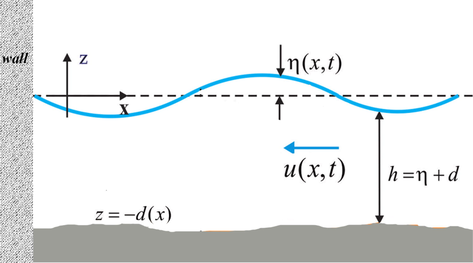

The sketch of the one-dimensional fluid flow in a semi-closed basin.

Export to PPT

The second condition involves Eq. (11). According to the nodal line position of the semi-closed basin in its fundamental mode described by Rabinovich et al. (2009), the water elevation at the basin mouth must be zero for all time. This results in the function $F(x)$ having a value of zero at $x=L$ , according to Eq. (5). It is mathematically written as

(14)

$$J_0\left(\frac{\omega L}{\sqrt{{\mathit{gh}}_1}}\right)=0\text{.}$$

Since our aim is to find the lowest natural frequency, we seek the smallest root of the Bessel function, that is

(15)

$$\frac{\omega L}{\sqrt{{\mathit{gh}}_1}}=2.4048,$$ where $\omega =2\pi /T_1$ for the fundamental resonant period $T_1$ . By rearranging the terms, we obtain. Fig. 2.

(16)

$$T_1=1.306\frac{2L}{\sqrt{{\mathit{gh}}_1}}\text{.}$$

Close

Fig. 2

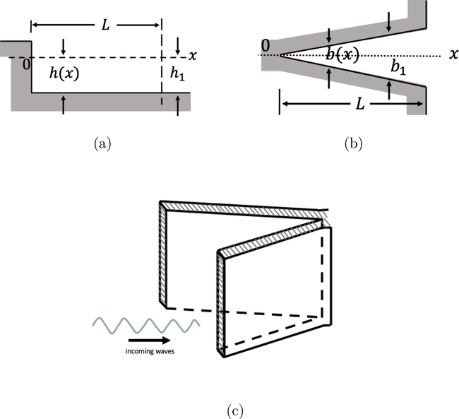
First basin configuration. (a) Longitudinal section (rectangular). (b) Top view of the basin (triangular). (c) Three-dimensional overview of basin configuration.

Export to PPT

3.2

3.2 Triangular longitudinal profile with triangular width

Now, we will analyse the second type of basin as shown in Fig. 3. The basin depth is increasing gradually following the function $h(x)=h_{1}x/L$ , whereas the basin width has the same configuration as in the previous subsection. Eq. (9) is then rewritten as follows

(17)

$${\omega }^{2}F+{\mathit{gF}}_x\left(\frac{2h_1}{L}\right)+{\mathit{gF}}_{\mathit{xx}}{h}_1\frac{x}{L}=0\text{.}$$

Close

Fig. 3

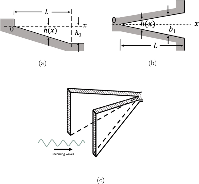
Second basin configuration. (a) Triangular longitudinal section. (b) Triangular basin width. (c) Three-dimensional visualization of the basin.

Export to PPT

The solution of Eq. (17) is

(18)

$$F(x)=\frac{1}{\sqrt{x}}\left(K_1{J}_1\left(2\omega \sqrt{\frac{\mathit{xL}}{{\mathit{gh}}_1}}\right)+K_2{Y}_1\left(2\omega \sqrt{\frac{\mathit{xL}}{{\mathit{gh}}_1}}\right)\right),$$ where $K_i,i=1,2$ are arbitrary constants. The first derivative of F with respect to x is

(19)

$$F_x(x)=\frac{1}{\sqrt{x^3}}\left[K_1(\gamma \sqrt{x}{J}_0(2\gamma \sqrt{x})-J_1(2\gamma \sqrt{x}))+K_2(\gamma \sqrt{x}{Y}_0(2\gamma \sqrt{x})-Y_1(2\gamma \sqrt{x}))\right],$$ where $\gamma =\omega \sqrt{L}/\sqrt{{\mathit{gh}}_1}$ .

The two conditions explained before hold for both types of basins discussed in this paper. Therefore, the following equation has to be satisfied

(20)

$$J_1\left(\frac{2\omega L}{\sqrt{{\mathit{gh}}_1}}\right)=0\text{.}$$

In order to find the non-trivial solution of the fundamental resonant period $T_1$ , we choose the nearest root of the Bessel function to the origin, which can be written as

(21)

$$\frac{2\omega L}{\sqrt{{\mathit{gh}}_1}}=3.8317\text{.}$$

Finally, the highest natural period of the second basin type is

(22)

$$T_1=1.640\frac{2L}{{\mathit{gh}}_1}\text{.}$$

Note that for both types of basins, the fundamental resonant periods are independent of the basin’s maximum width $b_1$ .

Table 1 summarizes our analytical results along with their relative errors when compared to the solutions obtained from the potential flow theory (Lamb, 1906). The relative error is calculated using $\left|\frac{T_1-T_1^{\ast }}{T_1^{\ast }}\right|$ , which is very small for both basin types (below 1 $\%$ ). It indicates that our mathematical model can be a good alternative to derive the basin’s natural period other than using potential flow theory, which is more complex to solve.

Table 1 Comparisons between the analytical fundamental resonant periods obtained using LSWE and potential flow theory.

Longitudinal section	$T_1$ (LSWE)	$T_1^{\ast }$ (potential flow theory)	Relative error
Rectangular	$1.306\frac{2L}{\sqrt{{\mathit{gh}}_1}}$	$1.308\frac{2L}{\sqrt{{\mathit{gh}}_1}}$	0.001529
Triangular	$1.640\frac{2L}{\sqrt{{\mathit{gh}}_1}}$	$1.653\frac{2L}{\sqrt{{\mathit{gh}}_1}}$	0.007864

4 Numerical method

This section provides the proposed numerical model to find the fundamental resonant period of the discussed basins. As depicted in Fig. 4, mass conservation Eq. (3) is stored within the green cells, while the other cells are used to calculate momentum balance Eq. (4). Hence, the half-grid points ( $x_{j+1/2}$ ) which are the center of momentum cells will contain the information of $u(x,t)$ , and the value of $\eta (x,t)$ is stored at full-grid points ( $x_j$ ). Similar to the wave elevation, $h(x)$ will also be calculated at full-grid points.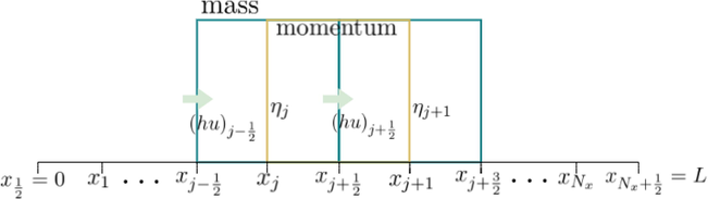

Close

Fig. 4

Illustration of finite volume method on a staggered grid.

Export to PPT

The constructed numerical scheme to simulate wave resonance in basins with varying width is

The symbol ${\eta }_j^n$ represents $\eta (x_j,t^n)$ , that is the free-surface elevation at $x=j\mathrm{\Delta }x$ ( $j=0,1,2,\dots ,N_x$ ) and $t=n\mathrm{\Delta }t$ ( $n=0,1,2,\dots ,N_t$ ). To satisfy the Courant-Friedrichs-Lewy stability condition, several parameters are chosen so that $(\mathrm{\Delta }t/\mathrm{\Delta }x)\sqrt{{\mathit{gh}}_{\max }}⩽1$ , for $g=9.81$ m/ $s^2$ .

5 Simulation results and discussion

Using the presented numerical scheme from the previous section, we ran several simulations to find the numerical fundamental resonant period of each basin. The parameters used for the simulations are: $L=25$ m; $h_1=1.5$ m; $b_1=1.5$ m; $\mathrm{\Delta }x=0.1$ ; and $\mathrm{\Delta }t=\mathrm{\Delta }x/\sqrt{{\mathit{gh}}_1}$ . The basin length and depth are chosen based on the shallow water criteria, that is, the total water depth must not exceed 1/20 of the wavelength. We observe the resonance phenomenon after 300 s at the basin boundary ( $x=0$ ).

To test whether the scheme (Eqs. (23)–(25)) can simulate the phenomenon well, we first try to observe the wave propagation using the analytical periods as depicted in Fig. 5. For both basin types, the numerical simulations using both analytical periods indicate an increment of the wave amplitude at $x=0$ over the time given, which characterizes a resonance. It shows that the numerical scheme is a good approximation for studying the phenomenon.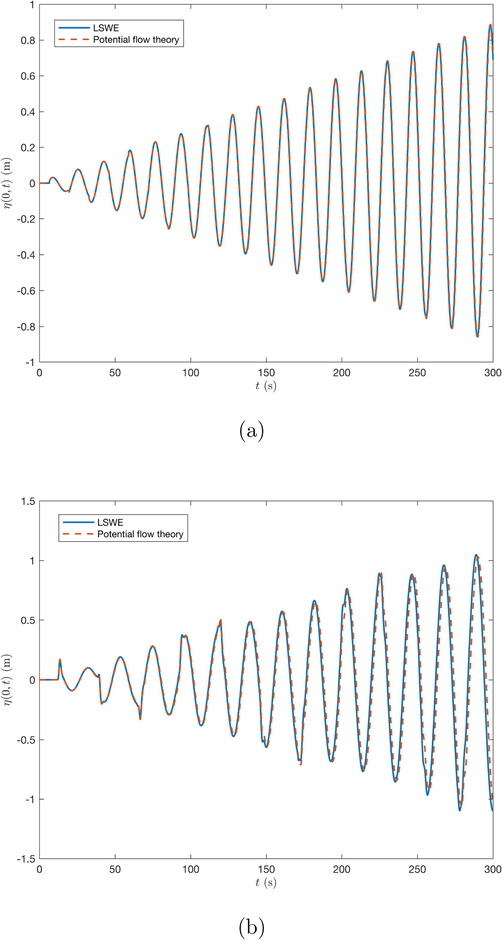

Close

Fig. 5

Resonance phenomenon in a rectangular (a) and triangular (b) basin with non-constant width using analytical fundamental resonant period derived from LSWE and potential flow theory (Table 1).

Export to PPT

Next, we conducted a numerical experiment to find the highest basins’ natural period. We use the sought analytical periods as our initial guess and then increase the values slowly until the wave amplitude becomes constant over time, meaning that the resonance no longer occurs. Hence, the maximum periods obtained are the fundamental resonant periods because they are the highest periods that can generate resonance. Table 2 shows the comparison between the obtained numerical periods ( ${\overline{T}}_1$ ) and analytical periods ( $T_1$ : LSWE and $T_1^{\ast }$ : potential flow theory). Since the relative errors are below 1 $\%$ , we can say that our numerical approach aligns with the analytical approximations.

Further, we also compared the wave amplitude rise due to resonance in basins with varying widths and constant width using data from (Magdalena et al., 2020). Fig. 6 presents the wave propagation in both basin types, while the details regarding the maximum wave amplitudes are given in Table 3. The resonance phenomena in basins with non-constant width produce higher maximum wave amplitudes. The difference is greater for the triangular basin compared to the rectangular one, as shown by the ratio numbers listed in Table 3.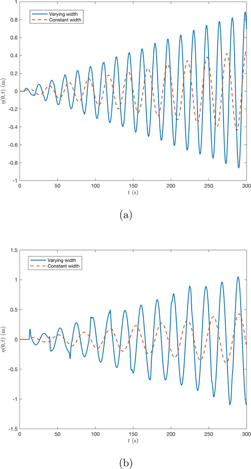

Close

Fig. 6

Resonance phenomenon in a rectangular (a) and triangular (b) basin with varying width compared to resonance in basin with constant width.

Export to PPT

These results are related to the fundamental resonant periods of both basin types. Overall, the periods of varying-width basins are lower than basins with constant width. As derived by Magdalena et al. (2020), the period of the constant-width rectangular basin is $2(2L/\sqrt{{\mathit{gh}}_1})$ which is 0.694 higher than the varying-width type. Since waves with lower periods carry more energy, the incoming waves generating resonance in varying-width basins will have greater amplitude. As a result, the maximum wave amplitude at the basin boundary will also be higher. On the other hand, the difference in the triangular basin is 0.9728. We can see that it is greater than the rectangular one and, thus, the ratio number showing the increment of the maximum wave amplitude is also higher for the triangular basin.

From these findings, one should be more aware of basins with triangular width, since the maximum wave elevation for this type is higher than for regular width. One way to be more aware of this basin type is by incorporating tools to the basin configuration that can dampen the effect of the resonance phenomenon such as breakwater, revetment, or porous media.

6 Conclusion

A modification of linear shallow water equations that includes the effect of varying widths has been applied to derive the fundamental resonant period in several basin types. The governing equations are solved analytically using the separation of variables method and numerically by applying the staggered finite volume method. According to the analytical results, the sought resonant periods align with the results obtained from the potential flow theory. Similar outcomes are also produced from numerical simulations. Since the simulations using the two analytical resonant periods indicate resonance phenomena, we conclude that the scheme can approximate the governing equations well and, thus, we proceed to find the numerical resonant periods using the scheme. As expected, the relative errors between the numerical and the two analytical resonant periods are below 1 $\%$ which shows that our numerical results align with the analytical ones. Furthermore, we also compared the resonance phenomenon that occurs in constant-width and varying-width basins. Since the resonant periods are lower for basins with non-constant width, the incoming waves causing the resonance will have higher energy. Therefore, a higher wave elevation is produced at the basin boundary.

References

- Analytical and numerical studies of resonant wave run-up on a plane structure. J. Phys: Conf. Ser.. 2019;1321:022079
- [CrossRef] [Google Scholar]
- An efficient covariant frame for the spherical shallow water equations: Well balanced dg approximation and application to tsunami and storm surge. Ocean Model.. 2022;169:101915
- Angle dependence in coupling conditions for shallow water equations at channel junctions. Computers Math. Appl.. 2022;108:49-65.
- Numerical simulation of dam-break problem using staggered finite volume method. AIP Conf. Proc.. 2016;1707(1):050003
- Experimental investigation on special modes with narrow amplification diagrams in harbor oscillations. Coast. Eng.. 2020;159:103720
- Hydrodynamics. Cambridge: University Press; 1906.
- Water waves resonance and its interaction with submerged breakwater. Results Eng.. 2022;13:100343
- Numerical modeling of 2d wave refraction and shoaling. AIP Conf. Proc.. 2014;1589(1):480-483.
- model for dam break over a movable bed using finite volume method, Int. J. Geomate. 2020;19(71):98-105. cited By 5
- Seiches and harbour oscillations in a porous semi-closed basin. Appl. Math. Comput.. 2020;369:124835
- Widowati: 1d–2d numerical model for wave attenuation by mangroves as a porous structure. Computation. 2021;9(6)
- Resonant periods of seiches in semi-closed basins with complex bottom topography. Fluids. 2021;6(5)
- Analytical and numerical studies for wave generated by submarine landslide. Alexandria Eng. J.. 2022;61(9):7303-7313.
- A staggered method for the shallow water equations involving varying channel width and topography. Int. J. Multiscale Comput. Eng.. 2018;16:231-244.
- [Google Scholar]
- Momentum conservative schemes for shallow water flows. East Asian J. Appl. Math.. 2014;4(2):152-165.
- Rabinovich, A., 2009. Chapter 9: Seiches and Harbor Oscillations in Handbook of Coastal and Ocean Engineering (edited by Y.C. Kim), World Scientific Publ., Singapore, pp. 193–236.
- An analytic investigation of oscillations within a harbor of constant slope. Ocean Eng.. 2011;38(2):479-486.
- Analytical solutions for oscillations in a harbor with a hyperbolic-cosine squared bottom. Ocean Eng.. 2014;83:16-23.
- Theoretical analysis of harbor resonance in harbor with an exponential bottom profile. China Ocean Eng. 2015;29:821-834.
- An analytical investigation of oscillations within a circular harbor over a conical island. Ocean Eng.. 2020;195:106711