

Translate this page into:
Construction of new exact solutions of the resonant fractional NLS equation with the extended Fan sub-equation method
⁎Corresponding author at: Department of Mathematics, Huzhou University, Huzhou 313000, PR China. chuyuming@zjhu.edu.cn (Yu-Ming Chu)
-
Received: ,
Accepted: ,
This article was originally published by Elsevier and was migrated to Scientific Scholar after the change of Publisher.
Peer review under responsibility of King Saud University.
Abstract
The fucus of this study is to find a set of some novel solutions concerning the resonant fractional nonlinear Schrödinger equation (R-FNLSE) with quadratic-cubic nonlinearity by employing the extended FAN sub-equation approach. The parameter is the core constraint which simulate the flow rate propagation, plays a key rote in telecommunications and the theory of optical fibres. This equation expresses the gesture of solitons and Madelung fluids in various nonlinear systems. These outcomes are optical, bright, dark, explicit, periodic and combined wave solutions and efficiently demonstrated with the aid of 3D plots. The representation of these solutions is carried out in order to have an idea about the structure of such model and can also be extended to many other complex models of recent era.
Keywords
Resonant fractional nonlinear Schrödinger equation
Extended Fan sub-equation method
New solutions

1 Introduction
In recent decades, it has been noticed that nonlinear phenomena have remarkable properties in physics and mathematical engineering. The phenomenon of nonlinear evaluation equations (NLEE) has received a lot of attention and has become one of the most interesting areas of research. Such type of models are widely used to elucidate many complex physical phenomena that occur in fluid and plasma wave mechanics, fiber optic communications, biophysics, Soliton’s theory, and many more (Kalim et al., 2018; Ghanbari et al., 2019a; Ghanbari et al., 2019b; Munusamy et al., 2020; Rezazadeh, 2018).
The area of nonlinear partial differential equations is becoming one of the most essential disciplines describing dynamics of key phenomena of nature and has attracted renowned researchers and scientists in the theory of optical fibre arising in telecommunications, spectroscopy, plasma physics and many more. Optical solitons are basically localized electromagnetic waves which can transmit large amount of information through optical fibers across the trans-oceanic distance in femto-seconds. In the modern era of science and technology, the theory of solitons has created revolutionary developments in the telecommunication engineering and is one of the most blistering field of research over the past few decades and reckon as the technology of future generation for high-speed communication systems (Ghanbari et al., 2020; Hosseini et al., 2020a; Hosseini et al., 2020b; Korpinar et al., 2019; Hashemi et al., 2019).
Many complex phenomena in diverse areas of nonlinear science are usually described by nonlinear models. One of the most famous of these nonlinear equations is the Schrödinger’s equation. This equation has been used in several domains among which: fiber optics, hydrodynamics, Plasma physics, nonlinear electrical transmission lines, and so on (Liu et al., 2019). However, there are a multitude of nonlinear equations such as the Ginzburg–Landau equation (Wazwaz, 2006), the Korteweg de Vries equation (Seadawy et al., 2020), the Zoomeron equation (Hosseini et al., 2020c), the Boussinesq equation (Mehdinejadiani and Parviz, 2020), to mention a few, that can also help to describe many systems. It’s worth mentioning that integer order derivatives are previously utilised to analyze these problems. However, in order to gain a better understanding of the dynamics of these nonlinear equations, a common type of derivative called fractional derivatives should be presented (Manafian and Lakestani, 2017; Miller and Ross, 1993).
This concept is a generalization of derivatives. Thus, we observe that the fractional NLEE is a natural extension of a NLEE of integeral order. These fractional differential equations are generally not easy to solve and methods that have been proposed in the literature to transform them are used. Among these methods, we can list the Caputo fractional derivatives, the Riemann–Liouville fractional derivatives, modified Riemann–Liouville derivative, conformable fractional derivative. The enactment of such methods is just a beginning for a revolution of recent era towards fractional calculus. To date, there are several methods in the literature that can be implemented to deal with the nonlinear models arising in diverse disciplines (Goswami et al., 2020; Singh et al., 2021a; Singh et al., 2021b; Singh et al., 2021c).
The outline of this study is given as follows: in Section 2, a brief introduction to the R-FNLSE with quadratic-cubic nonlinearity is illustrated whereas in Section 3 some noval anlytical solutions to the nonlinear complex model (1) are established. The geometrical behavior of the solutions is demonstrated in Section 4. At the end, the conclusions have been extracted.
2 The R-FNLSE with quadratic-cubic nonlinearity
Over the last few decades, the study solitonic and optical behaviour of nonlinear models is becoming one of the most excited topics in the diverse disciplines of contemporary science. Our prospective is applicable until the given model imply more even odd order partial derivative terms (Seadawy and Lu, 2017; Younis et al., 2020).
Over the last couple of years, many computational analysis have been established effectively to describe the soliton solutions of various type of nonlinear Schrödinger equation (NLSE) among these are, the extended sinh-Gordon equation expansion method (Baskonus et al., 2018), extended Jocobi’s elliptic approach (Hong and Lu, 2009), the modified auxiliary equation mapping method (Seadawy et al., 2020), the inverse scattering transformation method (Zhang and Chen, 2019), extended rational sine–cosine method (Mahak and Akram, 2019), and many more.
The purpose of the study is to investigate the NLSE of fractional order (Bhrawy et al., 2014) with quadratic-cubic nonlinearity, as well as perturbation terms and higher order dispersions (third and fourth order dispersions). The R-FNLSE with quadratic-cubic nonlinearity is studied by using extended Fan sub-equation (EFSE) approach.
3 Applications to the EFSE method
The transformation
The solution for Eq. (4) is of the fashion (Kalim et al., 2021; El-Wakil and Abdou, 2008)
Inserting Eq. (6) along Eq. (7) in Eq. (4) and picking the coefficients of ,
We select variables suitably which gives
We have soliton solutions
Case I
If , there may exist parameters , satisfy , the solutions of (1) are .
Type I.
,
,
. We obtain the dark optical solitons in the form as follows
We obtain the combined bright-dark optical soliton in the form as follows
We obtain the combined dark-singular optical solitons in the form as follows
Type II.
,
,
. The collection of periodic solitons are obtained
If
is one of the
. A collection of dark optical soliton is observed
, we have the following solution of (1) in the form .
Type I.
, where
are arbitrary constants.
, where
are arbitrary constants.
Eqs. (21), (22) give a set of bright and singular optical solitons for
, where
are arbitrary constants.
, where
are arbitrary constants.
Another class of dark and singular optical solitons is obtained for
, where
are arbitrary constants.
, where
are arbitrary constants.
, where
are arbitrary constants.
, Eq. (1) have solutions of the form .
Type I
,
,
4 Discussion and results
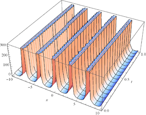
To display a set of novel travelling wave solutions to the Eq. (1), Mathematica 11.0 is executed to demonstrate the behaviour of bit flow and to understand the complex structure of solitons for a set of limitations. The parameter is the core constraint which simulate the flow rate propagation, plays a key rote in telecommunications and the theory of optical fibres.
Fig. 1 illustrates the solution
constructed in Case I (Type I) for
= −2,
= 0.1,
= 0.1,
= 0.5,
= 2,
= 2,
= 2,
= 1,
= 1,
= 2,
= 3,
= 5,
= 1,
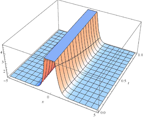
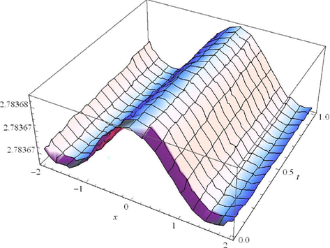
= 2, while Fig. 2 illustrates the solution
constructed in Case I (Type I) for
= −2,
= 0.1,
= −0.5,
= 1,
= 1,
= 2,
= 2,
= 1,
= 1,
= 2,
= 3,
= 3,
= 1,
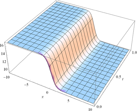
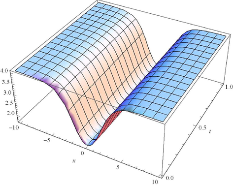
= 1, whereas Fig. 3 visualizes the solution
produced in Case I (Type I) for
= −2,
= 0.1,
= 0.1,
= 0.5,
= 2,
= 2,
= 2,
= 1,
= 1,
= 2,
= 3,
= 5,
= 3,
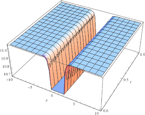
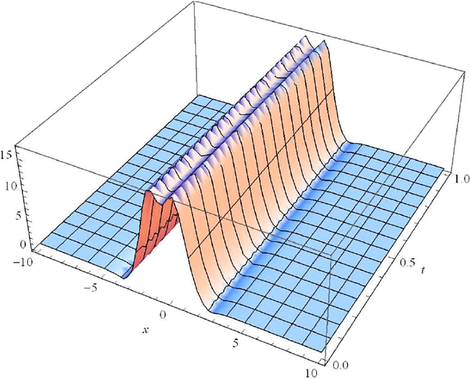
= 2. Similarly, Fig. 4 illustrates the solution
constructed in Case I (Type I) for
= −2,
= 0.1,
= 0.1,
= 0.5,
= 2,
= 2,
= 2,
= 2,
= 1,
= 2,
= 3,
= 3,
= 1,
= −1, while Fig. 5 visualizes the solution
constructed in Case I (Type II) for
= 0.1,
= 1,
= 0.1,
= 1,
= 2,
= 2,
= 2,
= 2,
= 1,
= 2,
= 1,
= 1,
= 1,
= 1.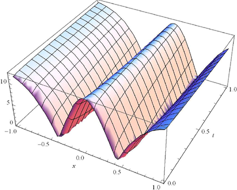
= −2,
= 0.1,
= 0.1,
= 0.5,
= 2,
= 2,
= 2,
= 1,
= 1,
= 2,
= 3,
= 5,
= 1,
= 2.
= −2,
= 0.1,
= −0.5,
= 1,
= 1,
= 2,
= 2,
= 1,
= 1,
= 2,
= 3,
= 3,
= 1,
= 1.
= −2,
= 0.1,
= 0.1,
= 0.5,
= 2,
= 2,
= 2,
= 1,
= 1,
= 2,
= 3,
= 5,
= 3,
= 2.
= −2,
= 0.1,
= 0.1,
= 0.5,
= 2,
= 2,
= 2,
= 2,
= 1,
= 2,
= 3,
= 3,
= 1,
= −1.
= 0.1,
= 1,
= 0.1,
= 1,
= 2,
= 2,
= 2,
= 2,
= 1,
= 2,
= 1,
= 1,
= 1,
= 1.
Comparably, Fig. 6 displays the solution
constructed in Case II (Type I) for
= −2,
= 0.1,
= 0.1,
= 0.5,
= 2,
= 2,
= 2,
= 2,
= 1,
= 2,
= 3,
= 0,
= −1,
= 1 whereas Fig. 7 reveals the solution
constructed in Case III (Type I) for
= −2,
= 0.1,
= 0.1,
= 0.5,
= 2,
= 2,
= 2,
= 2,
= 5,
= 2,
= 3,
= 1,
= 2,
= 3 and Fig. 8 displays the solution
constructed in Case III (Type I) for
= 1,
= 0.5,
= 0.1,
= 1,
= 2,
= 2,
= 2,
= 2,
= 1,
= 2,
= 3,
= 1,
= 2,
= 3.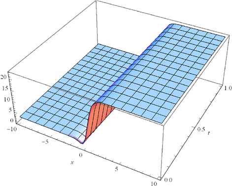
= −2,
= 0.1,
= 0.1,
= 0.5,
= 2,
= 2,
= 2,
= 2,
= 1,
= 2,
= 3,
= 0,
= −1,
= 1.
= −2,
= 0.1,
= 0.1,
= 0.5,
= 2,
= 2,
= 2,
= 2,
= 5,
= 2,
= 3,
= 1,
= 2,
= 3.
= 1,
= 0.5,
= 0.1,
= 1,
= 2,
= 2,
= 2,
= 2,
= 1,
= 2,
= 3,
= 1,
= 2,
= 3.
Likewise, Fig. 9 illustrates the solution
constructed in Case IV (
) for
= −2,
= 0.1,
= 0.1,
= 0.5,
= 2,
= 2,
= 2,
= 1,
= 1,
= 2,
= 3, while Fig. 10 represents the solution
constructed in Case IV (
) for
= −2,
= 0.1,
= 0.1,
= 0.5,
= 2,
= 2,
= 2,
= 1,
= 1,
= 2,
= 3.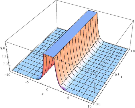
= −2,
= 0.1,
= 0.1,
= 0.5,
= 2,
= 2,
= 2,
= 1,
= 1,
= 2,
= 3.
= −2,
= 0.1,
= 0.1,
= 0.5,
= 2,
= 2,
= 2,
= 1,
= 1,
= 2,
= 3.
5 Conclusion
In this paper, the resonant fractional nonlinear Schrödinger equation with quadratic-cubic nonlinearity is investigated with the help of the conformable derivative associated to the extended FAN sub-equation method. The latest scientific computing tools is implemented to visualize the dynamics of the complex fractional model (1). The structure of the model is displayed for various set of parameters in an intensive way. To further analyze the behavior of the nonlinear fractional phenomenon, a number of significant solitons have been systematically identified, including bright, dark, singular, combination, optical, singular optical, and gloss-singular combination solitons, as shown in Figs. 1–10. The parameter is the core constraint which simulate the flow rate propagation, plays a key rote in telecommunications and the theory of optical fibres. The computational results are very encouraging, powerful, efficient and can also be extended to have advanced exact solutions for many complex models from different branches of engineering and applied sciences.
Availability of supporting data
Not applicable.
Funding
This work was supported by the National Natural Science Foundation of China (Grant Nos. 11971142, 11871202, 61673169, 11701176, 11626101, 11601485).
6 Author’s contributions
All authors contributed equally to the writing of this paper. All authors read and approved the final manuscript.
Acknowledgements
The authors would like to express their sincere thanks to the support of National Natural Science Foundation of China.
Declaration of Competing Interest
The authors declare that they have no known competing financial interests or personal relationships that could have appeared to influence the work reported in this paper.
References
- Investigations of dark, bright, combined dark-bright optical and other soliton solutions in the complex cubic nonlinear Scrödinger equation with d-potential. Superlatt. Microstruct.. 2018;115:19-29.
- [Google Scholar]
- Optical soliton perturbation with spatio-temporal dispersion in parabolic and dual-power law media by semi-inverse variational principle. Optik. 2014;125(17):4945-4950.
- [Google Scholar]
- The extended Fan sub-equation method and its applications for a class of nonlinear evolution equations. Chaos Solitons Fract.. 2008;36(2):343-353.
- [Google Scholar]
- Soliton solutions of the resonant nonlinear Schrödinger’s equation in optical fibers with time dependent coefficients by simplest equation approach. J. Mod. Opt.. 2013;60(19):1627-1636.
- [Google Scholar]
- Solitary wave solutions to the Tzitzeica type equations obtained by a new efficient approach. J. Appl. Anal. Comput.. 2019;9(2):568-589.
- [Google Scholar]
- The new exact solitary wave solutions and stability analysis for the (2+1)-dimensional Zakharov-Kuznetsov equation. Adv. Differ. Equ.. 2019;2019(1):1-15.
- [Google Scholar]
- Abundant solitary wave solutions to an extended nonlinear Schrödinger’s equation with conformable derivative using an efficient integration method. Adv. Differ. Equ.. 2020;2020(1):1-25.
- [Google Scholar]
- Numerical computation of fractional Kersten-Krasil-shchik coupled KdV-mKdV system occurring in multi-component plasmas. AIMS Math.. 2020;5(3):2346.
- [Google Scholar]
- Symmetry properties and exact solutions of the time fractional Kolmogorov-Petrovskii-Piskunov equation. Rev. Mex. de Fis.. 2019;65(5):529-535.
- [Google Scholar]
- New Jacobi elliptic functions solutions for the higher-order nonlinear Scrödinger equation. Int. J. Nonlinear Sci.. 2009;7(3):360-367.
- [Google Scholar]
- Soliton solutions of the Sasa-Satsuma equation in the monomode optical fibers including the beta-derivatives. Optik. 2020;224:165425
- [Google Scholar]
- New wave form solutions of nonlinear conformable time-fractional Zoomeron equation in (2+1)-dimensions. Waves Random Complex Media 2020:1-11.
- [Google Scholar]
- Optical solitons in monomode fibers with higher order nonlinear Schrödinger equation. Optik. 2018;154:360-371.
- [Google Scholar]
- New optical solitons for Biswas-Arshed equation with higher order dispersions and full nonlinearity. Optik. 2019;206:163332
- [Google Scholar]
- A variety of nonautonomous complex wave solutions for the (2+ 1)-dimensional nonlinear Schrödinger equation with variable coefficients in nonlinear optical fibers. Optik.. 2019;180:917-923.
- [Google Scholar]
- Exact solitary wave solutions by extended rational sine-cosine and extended rational sinh-cosh techniques. Phys. Scr.. 2019;94(11):115212
- [Google Scholar]
- A new analytical approach to solve some of the fractional-order partial differential equations. Indian J. Phys.. 2017;91:243-258.
- [Google Scholar]
- Analytical solutions of space fractional Boussinesq equation to simulate water table profiles between two parallel drainpipes under different initial conditions. Agric. Water Manag.. 2020;240:106324
- [Google Scholar]
- An Introduction to the Fractional Calculus and Fractional Differential Equations. New York: Wiley-Interscience Publication, Wiley; 1993.
- Existence of solutions for some functional integrodifferential equations with nonlocal conditions. Math. Methods Appl. Sci.. 2020;43(17) 30:10319-10331.
- [Google Scholar]
- New solitons solutions of the complex Ginzburg-Landau equation with Kerr law nonlinearity. Optik. 2018;167:218-227.
- [Google Scholar]
- Bright and dark solitary wave soliton solutions for the generalized higher order nonlinear Schrödinger equation and its stability. Results Phys.. 2017;7:43-48.
- [Google Scholar]
- Propagation of kink and anti-kink wave solitons for the nonlinear damped modified Korteweg-de Vries equation arising in ion-acoustic wave in an unmagnetized collisional dusty plasma. Physica A Stat. Mech. Appl.. 2020;544:123560
- [Google Scholar]
- An efficient computational approach for local fractional Poisson equation in fractal media. Numer. Methods Partial Differ.. 2021;37(2):1439-1448.
- [Google Scholar]
- An efficient numerical approach for fractional multidimensional diffusion equations with exponential memory. Numer. Methods Partial Differ.. 2021;37(2):1631-1651.
- [Google Scholar]
- Computable generalization of fractional kinetic equation with special functions. J. King Saud Univ. Sci.. 2021;33(1):101221
- [Google Scholar]
- Optical solitons and conservation laws with quadratic-cubic nonlinearity. Optik. 2017;128:63-70.
- [Google Scholar]
- Explicit and implicit solutions for the one-dimensional cubic and quintic complex Ginzburg-Landau equations. Appl. Math. Lett.. 2006;19(10):1007-1012.
- [Google Scholar]
- A variety of exact solutions to (2+1)-dimensional schrödinger equation. Waves Random Complex Media. 2020;30:490-499.
- [Google Scholar]
- Inverse scattering transformation for generalized nonlinear Schrödinger equation. Appl. Math. Lett.. 2019;98:306-313.
- [Google Scholar]


