

Translate this page into:
Computation of vertex and edge resolvability of benzenoid tripod structure
⁎Corresponding author.
-
Received: ,
Accepted: ,
This article was originally published by Elsevier and was migrated to Scientific Scholar after the change of Publisher.
Peer review under responsibility of King Saud University.
Abstract
In the chemistry, the chemical compound’s structures are commonly shown by the graphs. In the scenario, atoms are replaced with vertices or nodes and bond types with simple lines known as edges. When the each node and edge of a graph have distinct representation or location with respect to the chosen vertices in a subset from the graph is known as the resolving set of mixed metric dimension say . This concept is known as vertex and edge resolvability parameter. This concept is usually helps to acquired a unique location or position of a structure or a graph. It is used to know the patterns of different drugs in the pharmaceutical research. There are many other applications of this variant. The exact metric dimension or resolving set of mixed metric dimension of benzenoid tripod structure is found in this research work. We proved that, this parameter is constant for the particular structure of benzenoid tripod graph.
Keywords
05C12
05C90
05C05
Node-resolvability
Edge-resolvability
Benzenoid structure
Benzenoid tripod

1 Introduction
Understanding the chemical structures that support current chemical ideas, establishing and exploring unique mathematical models of chemical processes, and applying mathematical concepts and techniques to chemistry are just a few of the challenges that mathematical chemistry has lately addressed. Throughout the history of science, some countable researchers have been persuaded to utilize links between both major fields in which mathematics and the second most important is chemistry, as well as the prospect of using basic operations of arithmetic to deduce established and anticipate new chemical properties. Mathematical techniques are frequently employed in a variety of fields of physical chemistry, most notably thermodynamics and chemical energy. After physicists demonstrated in the early century that the main properties of chemical compounds could be foresee using the techniques of quantum theory, there was a considerable demand for math in chemistry. The realization that chemistry cannot be understood without understanding of quantum physics, including its sophisticated mathematical tools, was the fundamental driving factor that brought the math and its concepts into the laboratories of chemistry. We recommend various material for distinct studies of related to the topic of mathematical chemistry in th form of graph theory (Yang et al., 2019; Manzoor et al., 2020; Siddiqui et al., 2016).
To characterize the structural properties of clusters, polymers, crystals, processes, molecules and many other materials, chemical graph theory is used which is very deep and novel field of mathematical science. The nodes or vertices of this field can be orbitals, intermediates, group of atoms, molecule, electron and many other items. Some forces such as Debye, Keesom, van der Waals forces may all be used to show the relationships between a structure’s vertices, moreover, also some non-bonded and bonded connection, intermolecular bonding and basic reactions.
For the literature review and base case parameter of this case study, we will start from Nadeem et al. (2020), in which authors made a three-dimensional hexagonal structure and proved that the resolving set of this is constant, moreover this concept is named as locating number and discussed some applications. Particular type of chemical structure are also studied by this parameter, for example -boron nanotubes are discussed in Hussain et al. (2018), silicate star structure and its metric are determined in Simonraj and George (2015), on the cellulose network (Siddiqui and Imran, 2015). And another structure of nanotubes are reshaped with this parameter are available in Imran et al. (2019). Mixed metric generators for generalized Peterson graphs and some generalize classes of rotational symmetric graphs are studied in Raza and Ji (2020) and Raza et al. (2020). The graph generated from different path graphs and discussed its edge and vertex resolvability in Raza et al. (2020). The vertex and edge resolvability of polcyclic hydrocarbons from aromatic family are found in Azeem and Nadeem (2021).
The seminal paper of the notion of resolving sets, are available at Slater (1975), the same idea presented by Harary and Melter (1976) with the name of locating parameter. In the pure graph theoretical parameter (Chartrand et al., 2000; Chartrand et al., 2000) named it as metric generator. This parameter have distinct applications and implementations like, for determining the patterns of variant of drugs in the field of pharmaceutical research, the statement enclosed by Johnson (1993). Metric resolving parameters have different variant of applications, such as image processing, facility location problems, sonar and coastguard loran (Slater, 1975), combinatorial optimization (Sebö and Tannier, 2004), computer networks (Manuel et al., 2008), weighing problems (Söderberg and Shapiro, 1963), robot navigation (Khuller et al., 1996), for detailed and further study on this parameter see (Perc et al., 2013; Perc and Szolnoki, 2010). The notion of metric dimension is commonly employed to address many complex issues due to its vast range of applications. We refer to for resolvability parameters of various chemical structures (Hussain et al., 2018; Krishnan and Rajan, 2016; Siddiqui and Imran, 2014).
Two edges are separated in the similar manner of vertices. For example, instead of nodes of a graph two edges may have unique representation or locations in terms of with respect to the chosen vertices in a subset of a graph. Taking this reason behind (Kelenc et al., 2018) put forward another parameter known as the edge metric resolving set or the edge metric dimension. In which the used the metric of a graph in terms of edges to locate every pair of edges and it is purely depend on the selection of vertices. Later on Kelenc et al. (Dec 2017), developed a mixed metric dimension in which both notions (recognising vertices and edges) are combined, with the additional restriction that no two elements (vertices and edges) have the same distances with regard to the selected subset. For the computational costs of all above topics we suggested to see (Hauptmann et al., 2012; Lewis et al., 1983; Johnson, 1993; Johnson, 1998).
Next to this, some basic definitions are provided for the basic use of them in our main task. In the Section 2, construction of our main structure or chemical compound is drawn for the better understanding to readers. Also the same section included the results of main task in terms of lemmas and remarks. In the Section 3, conclusion is drawn and closing remarks are added. At the end appropriate references are given related to this research work.
Given below are basic concepts and background results related to study of this work.
Definition 1.1 Nadeem et al. (2020)
“Assume be an associated graph of chemical structure/network, whose vertex/node set we will denote with symbol or simply , while or is the edge/bond set, the shortest distance between two bonds denoted by , and calculated by counting the number of bonds while moving through the path. The distance between an edge , and a node is counted by the relation .”
Definition 1.2 Deng et al. (mar 2021)
“A vertex of a connected associated graph of a chemical structure, differentiates nodes ( ) and edges ( ), if . A subset is a mixed resolving set if any different pair of components of are separated by a node of . The minimum number of nodes in mixed resolving set for is named the mixed metric dimension and is denoted by . It is also known as blended version of both metric (Slater, 1975) and edge metric dimension (Chartrand et al., 2000).”
Theorem 1.3 Kelenc et al. (Dec 2017)
“If is the mixed metric dimension, then , iff is a path .”
2 Construction of tripod structure
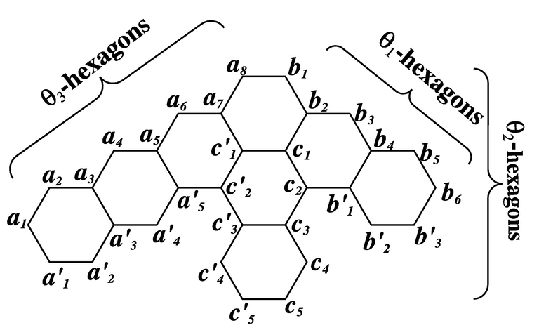
Benzenoid hydrocarbons are considered as very important and natural representations of graph of benzenoid systems, because of their prominence in theoretical chemistry (Chou et al., 2012). According to Ali et al. (2018), it is an established theory that benzenoids based hydrocarbons are vital and advantageous in the environmental, food and chemical sectors. Various catacondensed and pericondensed benzenoid structures were considered in respect to polynomial types. This is a tripod made of pericondensed benzenoid. It has nodes and bonds, with all the running parameters . In addition, Jamil et al. (2020) is available for comprehensive topological studies of benzenoid structures and in Koam et al. (2021), some metric based study is recently came up in the literature. The bond and node or we can say simply edge set and vertex set for this benzenoid structure is shown below. We use the labelling of edges and nodes provided in Fig. 1 in our primary results (Ali et al., 2021).
If is a benzenoid tripod graph with any of , then the mixed metric resolving set has minimum three members.
The order or the total amount of vertices in the benzenoid tripod’s associated graph with any of , are , and to look over the likelihood of mixed metric resolving set having three members in it, are . Over here we are focusing on three members in the set, from the result of Theorem 1.3 in the literature, the only two member of mixed metric resolving set is just for the basic graph f path. Now because of its computational cost of selecting mixed metric resolving set, for a graph, we can’t discover the precise number of mixed resolving sets, but from -possibilities we selected a subset and described as: . Proving of this claim that is also a subset having ability to be the candidate of mixed metric resolvability set of benzenoid tripod graph or , we will stick to 1.2’s definition. We will also look over the distinct placements or locations of each node and edge to meet the definition’s requirements, and the approach is explained above in Definition 1.2.
Positions with respect to , for the nodes with , are described as:
Positions with respect to , for the nodes with , are described as:
Positions with respect to , for the nodes with , are described as:
Positions with respect to , for the nodes with , are described as:
Positions with respect to , for the nodes with , are described as:
Positions with respect to , for the nodes with , are described as:
Given above are the positions of nodes only, with respect to the chosen vertices in , for the fulfillment of definition of mixed resolving set we still need to investigates the edges or bonds of graph. Following are positions of bonds that will complete the definition.
Positions with regard to , for the bonds with , are described as:
Positions with regard to , for the bonds with , are described as:
Positions with regard to , for the bonds with , are described as:
Positions with regard to , for the bonds with , are described as:
Positions with regard to , for the bonds with , are described as:
Positions with regard to , for the bonds with , are described as:
Positions with regard to , for the bonds with , are described as:
Positions with regard to , for the bonds with , are described as:
Positions with regard to , for the bonds with , are described as:
Positions of the joint edges are described as:
By the given positions of all -nodes and -edges of graph of benzenoid tripod with any of , with respect to , are unique and no two nodes, no two edges and not a single edge with a vertex have same position . As a result, we may infer that the nodes and edges of the graph have been resolved with only three nodes. So it is concluded that the members with minimality conditions of mixed metric resolving set of are three. □
If is a of benzenoid tripod graph with any of , then
As based on the definition of mixed metric dimension, the concept is solemnly based on the selected subset ( ) chooses in a manner that each edge and vertex have distinct location in regards to the chosen vertices in subset. The Lemma 2.1 shows and proved the chosen subset for the mixed metric resolving set and their hardness to be chosen with the condition of minimality. We proved in that lemma the subset is one of the candidate for the mixed metric resolving set for a particular benzenoid tripod or graph for all the possible combinatorial values of with any of . Moreover, we discussed in the same lemma that is fulfilling the minimality conditions on their members. It is impossible to get a subset with two members in a selected subset. It is sufficient to verify what we assert in the assertion that the mixed metric dimension of the benzenoid tripod is three, which concludes the proof. □
If is a benzenoid tripod graph with , then the mixed metric resolving set has minimum four members.
The order or the total amount of vertices in the benzenoid tripod’s associated graph with any of , are , and to look over the likelihood of mixed metric resolvability set having four members in it, are . Over here we are focusing on four members in the set, for the three cardinality of mixed resolving set we will discuss in next part of this proof. Now because of its computational cost of selecting mixed metric resolving set, for a graph, we can’t discover the precise number of mixed resolving sets, but from -possibilities we selected the subset and described as: . Proving of this claim that is also a subset having ability to be the candidate of mixed metric resolving set of benzenoid tripod graph or , we will stick to 1.2’s definition. We will also look over the distinct placements or locations of each node and edge to meet the definition’s requirements, and the approach is explained above in Definition 1.2.
Positions with respect to , for the nodes with , are described as:
Positions with respect to , for the nodes with , are described as:
Positions with respect to , for the nodes with , are described as:
Positions with respect to , for the nodes with , are described as:
Positions with respect to , for the nodes with , are described as:
Positions with respect to , for the nodes with , are described as:
Given above are the positions of nodes only, with respect to the chosen vertices in , for the fulfillment of definition of mixed resolving set we still need to investigates the edges or bonds of graph. Following are positions of bonds that will complete the definition.
Positions with respect to , for the bonds with , are described as:
Positions in regards to , for the bonds with , are described as:
Positions in regards to , for the bonds with , are described as:
Positions in regards to , for the bonds with , are described as:
Positions in regards to , for the bonds with , are described as:
Positions in regards to , for the bonds with , are described as:
Positions in regards to , for the bonds with , are described as:
Positions in regards to , for the bonds with , are described as:
Positions in regards to , for the bonds with , are described as:
Positions of the joint bonds are described as:
In support of a particular fact in order to meet the definition’s requirements of mixed metric resolving set, we can say that having four members in it is achievable, however when we discuss the optimized value of , we still have to look at the least number for . The given bellow are some scenarios to consider while determining whether is achievable or not. Though we have found the set of mixed metric resolvability by doing with the help of algorithm and satisfied that , but for the proving purpose we build some general cases and try to conclude that only is possible.
Case 1: Assume that , considering the constraint that, according to the demand of our theorem . In the same vertex’s position and/or edge’s position, the outcome is inferred and our supposition is contradicted by the fact that , where and . In the vertex’s position the similarities are in , where and .
Case 2: Assume that , considering the constraint that, according to the demand of our theorem . In the same vertex’s position and/or edge’s position, the outcome is inferred and our supposition is contradicted by the fact that , where and . In the vertex’s position the similarities are in , where and .
Case 3: Assume that , considering the constraint that, according to the demand of our theorem . In the same vertex’s position and/or edge’s position, the outcome is inferred and our supposition is contradicted by the fact that , where and . In the vertex’s position the similarities are in , where and .
Case 4: Assume that , considering the constraint that, according to the demand of our theorem . In the same vertex’s position and/or edge’s position, the outcome is inferred and our supposition is contradicted by the fact that , where and . In the vertex’s position the similarities are in , where and .
Case 5: Assume that , considering the constraint that, according to the demand of our theorem . In the same vertex’s position and/or edge’s position, the outcome is inferred and our supposition is contradicted by the fact that , where and . In the vertex’s position the similarities are in , where and .
Case 6: Assume that , considering the constraint that, according to the demand of our theorem . In the same vertex’s position and/or edge’s position, the outcome is inferred and our supposition is contradicted by the fact that , where . In the vertex’s position the similarities are in , where and .
Case 7: Assume that , considering the constraint that, according to the demand of our theorem . In the same vertex’s position and/or edge’s position, the outcome is inferred and our supposition is contradicted by the fact that , where and . In the vertex’s position the similarities are in , where and .
Case 8: Assume that , considering the constraint that, according to the demand of our theorem . In the same vertex’s position and/or edge’s position, the outcome is inferred and our supposition is contradicted by the fact that , where and . In the vertex’s position the similarities are in , where and .
Case 9: Assume that , considering the constraint that, according to the demand of our theorem . In the same vertex’s position and/or edge’s position, the outcome is inferred and our supposition is contradicted by the fact that , where and . In the vertex’s position the similarities are in , where and .
Case 10: Assume that , considering the constraint that, according to the demand of our theorem . In the same vertex’s position and/or edge’s position, the outcome is inferred and our supposition is contradicted by the fact that , where and . In the vertex’s position the similarities are in , where and .
Case 11: Assume that , considering the constraint that, according to the demand of our theorem . In the same vertex’s position and/or edge’s position, the outcome is inferred and our supposition is contradicted by the fact that , where and . In the vertex’s position the similarities are in , where and .
Case 12: Assume that , considering the constraint that, according to the demand of our theorem . In the same vertex’s position and/or edge’s position, the outcome is inferred and our supposition is contradicted by the fact that , where and . In the vertex’s position the similarities are in , where and .
Case 13: Assume that , considering the constraint that, according to the demand of our theorem . In the same vertex’s position and/or edge’s position, the outcome is inferred and our supposition is contradicted by the fact that , where and . In the vertex’s position the similarities are in , where and .
Case 14: Assume that , considering the constraint that, according to the demand of our theorem . In the same vertex’s position and/or edge’s position, the outcome is inferred and our supposition is contradicted by the fact that , where and . In the vertex’s position the similarities are in , where and .
Case 15: Assume that , considering the constraint that, according to the demand of our theorem . In the same vertex’s position and/or edge’s position, the outcome is inferred and our supposition is contradicted by the fact that , where and . In the vertex’s position the similarities are in , where .
Case 16: Assume that , considering the constraint that, according to the demand of our theorem . In the same vertex’s position and/or edge’s position, the outcome is inferred and our supposition is contradicted by the fact that , where and . In the vertex’s position the similarities are in , where .
Case 17: Assume that , considering the constraint that, according to the demand of our theorem . In the same vertex’s position and/or edge’s position, the outcome is inferred and our supposition is contradicted by the fact that , where and . In the vertex’s position the similarities are in , where and .
Case 18: Assume that , considering the constraint that, according to the demand of our theorem . In the same vertex’s position and/or edge’s position, the outcome is inferred and our supposition is contradicted by the fact that , where . In the vertex’s position the similarities are in , where and .
Case 19: Assume that , considering the constraint that, according to the demand of our theorem . In the same vertex’s position and/or edge’s position, the outcome is inferred and our supposition is contradicted by the fact that , where . In the vertex’s position the similarities are in , where and .
Case 20: Assume that , considering the constraint that, according to the demand of our theorem . In the same vertex’s position and/or edge’s position, the outcome is inferred and our supposition is contradicted by the fact that , where . In the vertex’s position the similarities are in , where .
Case 21: Assume that , considering the constraint that, according to the demand of our theorem . In the same vertex’s position and/or edge’s position, the outcome is inferred and our supposition is contradicted by the fact that , where . In the vertex’s position the similarities are in , where .
By the given positions of all -nodes and -edges of graph of benzenoid tripod with , in regards to , are unique and no two nodes, no two edges and not a single edge with a vertex have same position . As a result, we may infer that the nodes and edges of have been resolved with four vertices. We also checked that the mixed resolving set with are resulted in with either two edges, two vertices or a single edge with a vertex have same position .As a result, we may infer that the nodes and edges of with four vertices. It is finalized that the subset of mixed metric resolvability has minimal members and the graph has cardinal mixed metric dimension. □
If is a benzenoid tripod graph with , then
As based on the definition of mixed metric dimension, the concept is solemnly based on the selected subset ( ) chooses in a manner that each edge and vertex have distinct location in regards to the chosen vertices in subset. The Lemma 2.2 shows and proved the chosen subset for the mixed metric resolving set and their hardness to be chosen with the condition of minimality. We proved in that lemma the subset is one of the candidate for the mixed metric resolving set for a particular benzenoid tripod or graph for all the possible combinatorial values of with any of . Moreover, we discussed in the same lemma that is fulfilling the minimality conditions on their members. It is impossible to get a subset with three members in a selected subset. It is sufficient to verify what we assert in the assertion that the mixed metric dimension of the benzenoid tripod is three, which concludes the proof. □
- Benzenoid Tripod with
.
3 Conclusion
The study of intricate chemical networks and structures in their most fundamental forms has become easier thanks to only the field of mathematical chemistry, particularly graph theoretical chemistry. Resolvability is a parameter that controls how the whole node and edge set reconfigures itself into distinct ensembles to called or accessed them. A parameter having this feature is called as the mixed metric dimension, which transforms each node and edge of a structure into a unique shape. In this paper, we look at the benzenoid tripod structure in order to find the smallest edge and node combined resolving set. For this structure, we determined that the node and edge combined resolving set has a constant and precise number of members. In the scope of future work, this work can be done for any regular polygons instead of hexagons. This direction will be quite interesting and this help for readers.
Declaration of Competing Interest
The authors declare that they have no known competing financial interests or personal relationships that could have appeared to influence the work reported in this paper.
References
- Ahmad, Ali, Husain, Sadia, Azeem, Muhammad, Elahi, Kashif, Siddiqui, M.K., 2021. Computation of edge resolvability of benzenoid tripod structure 2021, 1–8.
- M-polynomials and topological indices of zigzagand rhombic benzenoid systems. Open Chem.. 2018;16(73–78):122-135.
- [Google Scholar]
- Metric-based resolvability of polycyclic aromatic hydrocarbons. Eur. Phys. J. Plus. 2021;136(395)
- [Google Scholar]
- Resolvability in graphs and the metric dimension of a graph. Discrete Appl. Math.. 2000;105:99-113.
- [Google Scholar]
- Zhang–zhang polynomials of various classes of benzenoid systems. MATCH Commun. Math. Comput. Chem.. 2012;68:31-64.
- [Google Scholar]
- On the edge metric dimension of different families of möbius networks. Math. Probl. Eng.. 2021;2021:1-9.
- [Google Scholar]
- Approximation complexity of metric dimension problem. J. Discrete Algorithms. 2012;14:214-222.
- [Google Scholar]
- Computing metric dimension and metric basis of lattice of alpha-boron nanotubes. Symmetry. 2018;10
- [Google Scholar]
- Computing the upper bounds for the metric dimension of cellulose network. Appl. Math. E-notes. 2019;19:585-605.
- [Google Scholar]
- Structure-activity maps for visualizing the graph variables arising in drug design. J. Biopharm. Stat.. 1993;3:203-236.
- [Google Scholar]
- Browsable structure-activity datasets, advances in molecular similarity. JAI Press Connecticut; 1998. p. :153-170.
- Uniquely identifying the edges of a graph: the edge metric dimension. Discrete Appl. Math.. 2018;251:204-220.
- [Google Scholar]
- Metric and fault-tolerant metric dimension of hollow coronoid. IEEE Access. 2021;9:81527-81534.
- [Google Scholar]
- Fault-tolerant resolvability of certain crystal structures. Appl. Math.. 2016;7:599-604.
- [Google Scholar]
- Computers and intractability: a guide to the theory of np-completeness. J. Symb. Log.. 1983;48(2):498-500.
- [Google Scholar]
- On minimum metric dimension of honeycomb networks. J. Discrete Algorithms. 2008;6(1):20-27.
- [Google Scholar]
- On entropy measures of polycyclic hydroxychloroquine used for novel coronavirus (covid-19) treatment. Polycyclic Aromat. Compd. 2020
- [Google Scholar]
- The locating number of hexagonal möbius ladder network. J. Appl. Math. Comput. 2020
- [Google Scholar]
- Evolutionary dynamics of group interactions on structured populations: a review. J. R. Soc. Interface. 2013;10(80)
- [Google Scholar]
- Computing the mixed metric dimension of a generalized petersengraph . Front. Phys.. 2020;8:211.
- [Google Scholar]
- On mixed metric dimension of some path related graphs. IEEE Access. 2020;8:188146-188153.
- [Google Scholar]
- On mixed metric dimension of rotationally symmetric graphs. IEEE Access. 2020;8:11560-11569.
- [Google Scholar]
- Computing metric and partition dimension of 2-dimensional lattices of certain nanotubes. J. Comput. Theor. Nanosci.. 2014;11(12):2419-2423.
- [Google Scholar]
- Computing the metric and partition dimension of h-naphtalenic and vc5c7 nanotubes. J. Optoelectron. Adv. Mater.. 2015;17:790-794.
- [Google Scholar]
- Computing topological indices of certain networks. J. Optoelectron. Adv. Mater.. 2016;18:9-10.
- [Google Scholar]
- On the metric dimension of silicate stars. In: ARPN J. Eng. Appl. Sci.. 2015. p. :2187-2192.
- [Google Scholar]
- Slater, P.J., 1975. Leaves of trees. In: Proceeding of the 6th Southeastern Conference on Combinatorics, Graph Theory, and Computing, Congressus Numerantium, vol. 14, pp. 549–559.


