

Translate this page into:
Comparative analysis for partial slip flow of ferrofluid nanoparticles in a semi-porous channel
⁎Corresponding author. jafar.buic@bahria.edu.pk (J. Hasnain)
-
Received: ,
Accepted: ,
This article was originally published by Elsevier and was migrated to Scientific Scholar after the change of Publisher.
Peer review under responsibility of King Saud University.
Abstract
The present study develops the equations that govern a steady flow of ferrofluid in a semi-porous channel (SPC) under the effects of Lorentz force. Three different base fluids namely water, kerosene and blood and magnetite as ferroparticles are used in the analysis. These equations are modeled by using the Cartesian coordinate system with the help of Berman’s similarity transformation. The partial slip condition is also considered at the lower plate of the channel. Three different methods of solution, namely the method of homotopy analysis (HAM) (analytical technique), the method of differential transformation (DTM) (semi-numerical technique) and the method of Runge-Kutta (numerical technique), are used to achieve the solution of non-dimensional, non-linear ordinary differential equations. For HAM solution, the auxiliary parameter delivers an effective way to regulate the convergence range of solution series whereas in DTM an approximation to the solution is obtained without any auxiliary parameter. The impact of Hartman and Reynolds number on the flow velocity are shown graphically and discussed. Finally, the comparison between the solution methods is given and found in very good agreement.
Keywords
Ferrofluid
Semi-porous channel
Magnetohydrodynamic
Velocity slip
DTM
HAM

Nomenclature
spatial coordinates []
velocity vector components in and directions, respectively []
hydrostatic pressure []
dimensionless variables [–]
dimensionless velocity components in and directions, respectively [–]
transpiration velocity
characteristic length []
constant magnetic field []
channel’s width []
slip length []
dimensionless velocity [–]
Hartmann number []
Reynolds number [–]
dimensionless pressure []
velocity of plate []
density []
dynamic viscosity []
electrical conductivity []
kinematic viscosity []
Nano–particle volume fraction [–]
ratio of and [–]
slip parameter []
Greek Symbols
nanofluid
base fluid
nano-solid particles
Subscripts
1 Introduction
Liquid streaming through semi-porous channel carries the significant number of utilization in biological and medical mechanisms like dialysis of blood in the synthetic kidney, blood circulation in capillaries, streaming in blood oxygenators and also in numerous engineering processes that include the designing of filters, composition of the porous/semi-porous pipes and gaseous diffusion. The foremost analysis on the fluid streaming in a channel was performed by (Berman, 1953)). Exact solutions of flow equations for the steady laminar flow in a rectangular channel with two porous walls were presented in this paper. Rashidi et al. (2010) studied the laminar flow of a non-Newtonian (micro-polar) fluid along a channel with porous boundaries and found the solution by a DTM. Shekholeslami et al. (2012) studied the flow of electrically conducting fluid in an SPC by the optical Homotopy Asymptotic method. The theoretical study of laminar nanofluid flowing through an SPC placed against a transverse magnetic field has been carried out by (Sheikholeslami et al., 2013; Abdel-Rahim and Rahman, 2014) computed the analytical and numerical solutions for the laminar flow of viscous fluid in an SPC. The mass transfer analysis of chemically reactive and electrically conducting second grade fluid streaming in an SPC was performed by Abbas et al., (2016). Using a parameterized perturbation method, (Abbas et al., 2018) investigated heat transfer for a two-dimensional steady flow of Maxwell fluid flowing in an axisymmetric SPC.
Scientists and engineers definitely have an urge to create advanced liquid varieties due to growing technological innovations, which should be more realistic in terms of heat exchange capacity. Nanofluid was developed by the dissemination of nano-sized particles in low thermal conductive liquids. This advanced fluid group, initially set up by Choi (Choi and Eastman, 1995; Choi et al., 2001), has both unique chemical and physical properties. Ferrofluid is also part of this fluid category. Ferrofluid is a mixture of ferrum (like ) and liquid that suspends multi-domain nanoparticles, coated with surfactants to reduce the surface tension between solid particles and traditional fluid. If there is no magnetic force in the vicinity of these particles, they behave like normal metallic particles. On the other side, in the presence of a magnetic force, these particles are briefly magnetized. A magnetic field can influence the location of the fluid because ferrofluid responds to an external magnetic field. Ferrofluid comprises of extremely small particles and in the presence of magnetic flux, they cannot settle with time and stay in their place. Few of the studies regarding the ferrofluid flow with different flow geometries are listed (Ghasemian et al., 2015; Abbas and Hasnain, 2017; Koriko et al., 2018; Salehpour and Ashjaee, 2019; Mousavi et al., 2020).
A powerful semi-numerical approach in accordance with the expansion of the Taylor series, (Zhou, 1986) primarily formulated DTM for linear and non-linear issues emerging in electrical engineering. In terms of unknown and known boundary conditions, this procedure quickly gives the precise value of the nth derivative of an analytical function at a point. For partial differential equations, DTM was established by Chen and Ho (1999) and for nonlinear ordinary differential equations, this method was employed by (Ayaz, 2004). The equations governing the biological flow problem have also been solved by DTM (Rashidi et al., 2011; Bég et al., 2013). Therefore, the main aim of this study is to analyze the numerical and semi-numerical solutions for the slip flow of ferrofluid nanoparticles in SPC with water and kerosene as based fluids. The partial slip condition is introduced at the lower moving wall plate of the channel. The final dimensionless form of equations for the velocity of fluid are solved using three different techniques homotopy analysis technique (homotopic solution), differential transform method (semi-numerical solution) and shooting method (numerical solution). Finally, the comparison of these methods and the effects of involving parameters of the velocity of fluid have been analyzed and discussed.
2 Detailing of the problem
The fluid under consideration is confined to a region between two parallel plates separated by a distance (see Fig. 1). A rigid infinite plate of length along -axis is placed at where the slip condition is applied, however, the other infinite plate is porous at which the transpiration velocity is The flow is steady, laminar and two-dimensional with constant physical properties of the fluid. Two different base fluids namely water and kerosene are considered carrying magnetite as nanoparticles. The intensity of a homogenous magnetic field is considered which is imposed transversely to the flow direction. The low magnetic Reynolds number assumption is also applied due to which induced magnetic field is neglected. The flow equations governing the flow phenomena under the above said suppositions are (Parsa et al., 2013; Mousavi et al., 2020)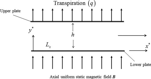
Graphical representation of the problem.
(Brinkman, 1952) provided the effective dynamic viscosity aswhere (<0.05 for most of the practical cases) signifies the volume fraction of nanoparticles. The particles can be of spherical or non-spherical shape. The effective density is given as (Mousavi et al., 2020)
Table 1 displays the physical properties of the base fluid and magnetic nanoparticle.
Physical property
Water
Kerosene
Blood
Density
997
783
1050
5180
Viscosity
0.001003
0.00164
0.003–0.004
–
The applicable boundary conditions (BCs) per situation are given by
Various technological and industrial applications, where the flow is enclosed by walls, pipes, and curved surfaces have motivated the researchers to use this Navier velocity slip condition at the walls. Few studies using this boundary condition are listed here (Abbas et al., 2016, 2017; Ashmawy, 2015; Ghosh et al., 2015; Sanyal and Sanyal, 1989).
The mean velocity can be computed by using the following relation
For similar solutions, we employ the following non-dimensional variables
Using the transformations defined in Eqs. (6), Eq. (1) - Eq. (3) are converted
Employing the above relations in Eq. (9) shows that the quantity independent of longitudinal variable Also from Eq. (8), it is found that is not a function of For simplicity we ignore the asterisks and after separating the variables, we have
Differentiate Eq. (11) with respect to one can obtain
The BCs are
Homotopy solution
Eqs. (13) and (12) are solved by using HAM, we choose the initial approximations given a
The linear operators are defined by
The curves are sketched for distinct values of fluid parameters at various orders of approximation to verify the convergence region of the solution, as suggested by Liao (2003). From Fig. 2(a), the convergence ranges of curves for at order 5 and 10 are and respectively, when and value of is In Fig. 2(b), curves convergence ranges for at orders 5 and 10 are and respectively, when and In Fig. 3(a, b) curves are plotted for and by taking along with From Fig. 3(a) the convergence range of curve for at 10th order is when the convergence range of curve at 10th order is when Similarly in Fig. 3(b) the convergence range of curve for at 10th order is when 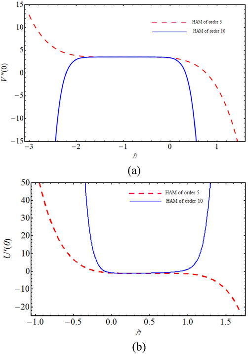
The curves of (a) and (b) stated by a different order of approximate solutions when
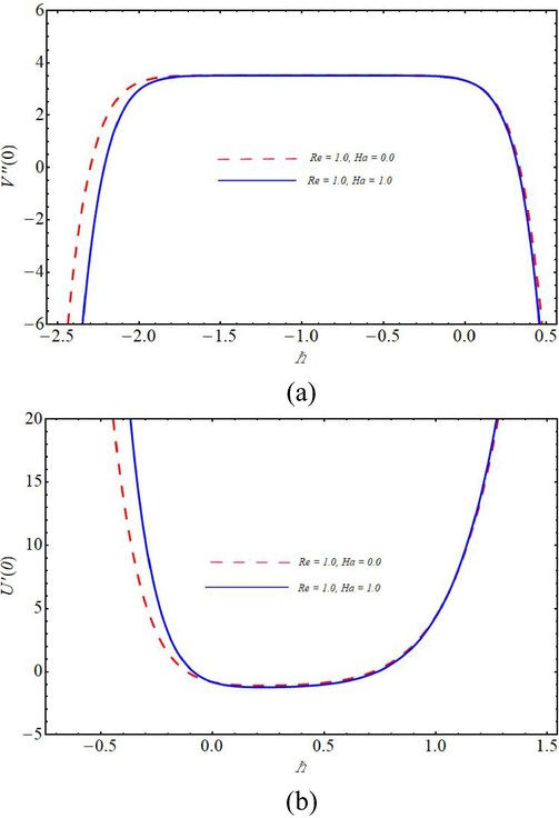
The curves of (a) and (b) stated by approximation solution of 10th order for when
3 Differential transform method
The kth derivative transformation of a function in one variable can be written as
By taking the differential transformation (DT) of the Eq. (13) the following transformation is obtained
denotes the DT of
The transform BCs are
We simultaneously solve Eq. (26) and (27) and obtained the values of and
Similarly, we use the DT of the (12) we have
In such a manner, we can easily solve Eqs. (24) and (28), by using direct command “NSolve” of MATHEMATICA, and able to find the values of
4 Results and discussion
To figure out velocity fields and we solved Eqs. (12) and (13) with respect to Eqs. (14) and (15) analytically by using HAM and DTM. Using the shooting process together with the Runge-Kutta technique, the numerical solution is additionally acquired. We plotted as well as to track the various impacts of the parameters involved. Fig. 4 compares velocity profiles at different orders of HAM along with the shooting method by taking fixed values of and Fig. 5 presents profiles of along with as well as bears comparisons of solutions by HAM upto10th-order approximation with DTM up to 20th-order approximation and the numerical solution with and It is found from these figures that results of HAM and DTM are incredibly correlated with the numerical results which clearly ensures the credibility of these methods.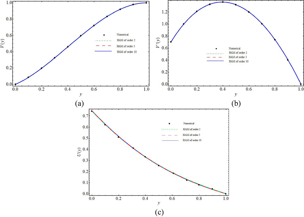
Comparison of (a) (b) and (c) attained at different orders of HAM with numerical solution, where
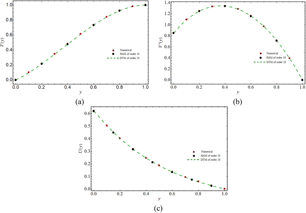
Comparison of numerical result with results of HAM and DTM for (a) (b) and where
Fig. 6 shows the variation in and for different values of with and for both slip and no-slip boundary conditions. A boost in the values of consequently increases the lateral mass flux at the upper plate due to which fluid approaches the upper plate. By means of this movement, the velocity in direction raises whereas it reduces in direction. From Fig. 6(a) and (c) one can easily observe that the velocity component in direction increases while the velocity distribution in direction decreases when the values of changes from 1 through 10 to 20. It can be seen from Fig. 6(b) that initially dimensionless transverse shear stress component increases with an increase in but reverse behavior is observed when we moved towards the upper plate. Fig. 6 also shows that the influence of is the same for both slip and no-slip boundary conditions. Fig. 7 depicts that the increasing values of decreases the fluid velocity distributions. But this decrement is more in Since the magnetic field is applied in the y-direction, therefore the component of Lorentz force will be created in direction. Consequently, the magnetohydrodynamic pull will not significantly affect and Whereas considerable change occurs in Fig. 8 presents the effect of volume fraction of ferro particles and slip parameter on fluid velocity distributions and Likewise also have a reverse behavior on near the lower and upper plates for both slip and no-slip boundary conditions.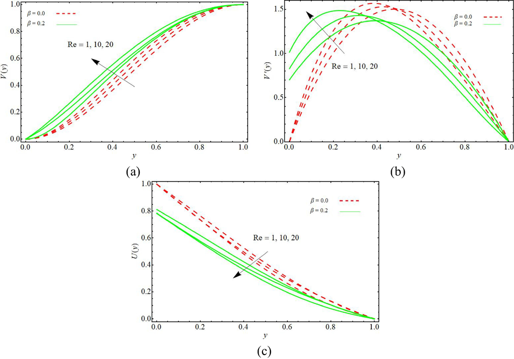
The profiles (a) (b) and (c) attained by the 10th –order approximation of the HAM for different value of and where
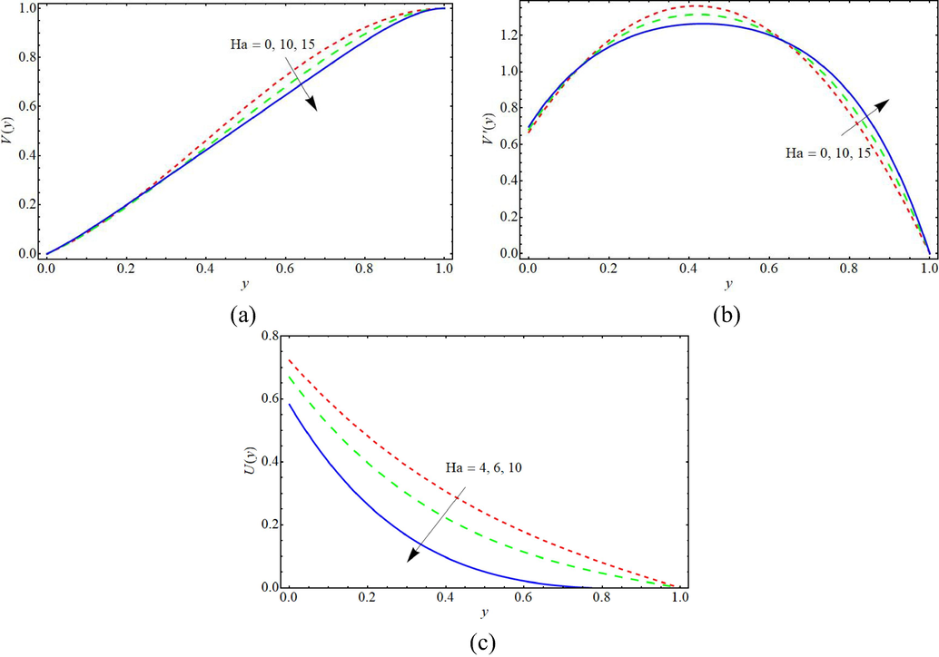
The profiles (a) (b) and (c) attained by the 10th –order approximation of the HAM for different value of where
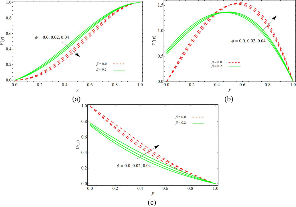
The profiles (a) (b) and (c) attained by the 10th –order approximation of the HAM for different value of and where
Outcomes of the present investigation are also tabulated through Tables 2–4. These tables reveal that the approximations of HAM upto10th-order and DTM up to 20th-order closely converges to the numerical values of velocity components and for different values of The calculations showed that the size of a solution in DTM is much less than HAM which can be observed from CPU time as shown in Table 2. These tables also show the comparison of these values for three different types of base fluid i.e. pure water, kerosene and blood.
Water base
Kerosene base
CPU time (s)
300.60
14.33
0.09
391.43
23.81
0.13
HAM of order 10
DTM of order 20
Numerical solution
HAM of order 10
DTM of order 20
Numerical solution
0
0.000000
0.000000
0.000000
0.000000
0.000000
0.000000
0.1
0.097758
0.097758
0.097758
0.097935
0.097935
0.097935
0.2
0.215311
0.215312
0.215311
0.215663
0.215664
0.215664
0.3
0.344742
0.344742
0.344742
0.345229
0.345229
0.345229
0.4
0.478699
0.478699
0.478699
0.479257
0.479258
0.479257
0.5
0.610245
0.610246
0.610245
0.610801
0.610801
0.610801
0.6
0.732703
0.732703
0.732703
0.733185
0.733186
0.733185
0.7
0.839514
0.839515
0.839514
0.839869
0.839870
0.839869
0.8
0.924121
0.924122
0.924121
0.924323
0.924324
0.924323
0.9
0.979879
0.979880
0.979879
0.979942
0.979943
0.979942
1
1.00000
1.00000
1.000000
1.000000
1.000000
1.000000
Blood Base
CPU time (s)
362.72
28.94
0.17
HAM of order 10
DTM of order 20
Numerical solution
0
0.000000
0.000000
0.000000
0.1
0.097725
0.097725
0.097725
0.2
0.215246
0.215246
0.215246
0.3
0.344651
0.344651
0.344651
0.4
0.478595
0.478595
0.478595
0.5
0.610141
0.610142
0.610142
0.6
0.732613
0.732613
0.732613
0.7
0.839447
0.839448
0.839448
0.8
0.924084
0.924084
0.924084
0.9
0.979867
0.979868
0.979868
1
1.000000
1.000000
1.000000
Water base
Kerosene base
HAM of order 10
DTM of order 20
Numerical solution
HAM of order 10
DTM of order 20
Numerical solution
0
0.850514
0.850517
0.850517
0.852112
0.852115
0.852114
0.1
1.090297
1.090300
1.090298
1.092136
1.092140
1.092138
0.2
1.247588
1.247589
1.247588
1.249195
1.249196
1.249194
0.3
1.328792
1.328792
1.328791
1.329851
1.329851
1.329849
0.4
1.338814
1.338814
1.338812
1.339160
1.339160
1.339159
0.5
1.281006
1.281006
1.281005
1.280612
1.280612
1.280611
0.6
1.157239
1.157239
1.157239
1.156200
1.156201
1.156200
0.7
0.968071
0.968072
0.968072
0.966606
0.966606
0.966607
0.8
0.713010
0.713010
0.713011
0.711465
0.711464
0.711466
0.9
0.390836
0.390834
0.390837
0.389714
0.389711
0.389715
1
0.000000
0.000000
0.000000
0.000000
0.000000
0.000000
Blood Base
HAM of order 10
DTM of order 20
Numerical solution
0
0.850220
0.850222
0.850221
0.1
1.089957
1.089959
1.089957
0.2
1.247290
1.247291
1.247290
0.3
1.328594
1.328596
1.328594
0.4
1.338748
1.338749
1.338748
0.5
1.281077
1.281078
1.281078
0.6
1.157431
1.157431
1.157431
0.7
0.968344
0.968344
0.968344
0.8
0.713298
0.713297
0.713298
0.9
0.391045
0.391042
0.391045
1
0.000000
0.000000
0.000000
Water base
Kerosene base
HAM of order 10
DTM of order 20
Numerical solution
HAM of order 10
DTM of order 20
Numerical solution
0
0.620077
0.620077
0.620077
0.617746
0.617746
0.617746
0.1
0.502367
0.502367
0.502367
0.499374
0.499374
0.499374
0.2
0.401721
0.401721
0.401721
0.398319
0.398319
0.398319
0.3
0.316599
0.316599
0.316599
0.313049
0.313049
0.313049
0.4
0.245171
0.245171
0.245171
0.241708
0.241708
0.241708
0.5
0.185479
0.185479
0.185479
0.182304
0.182304
0.182304
0.6
0.135577
0.135577
0.135577
0.132850
0.132850
0.132850
0.7
0.093624
0.093624
0.093624
0.091467
0.091467
0.091467
0.8
0.057961
0.057961
0.057961
0.056463
0.056463
0.056463
0.9
0.027150
0.027150
0.027150
0.026376
0.026376
0.026376
1
0.000000
0.000000
0.000000
0.000000
0.000000
0.000000
Blood Base
HAM of order 10
DTM of order 20
Numerical solution
0
0.620511
0.620511
0.620511
0.1
0.502924
0.502924
0.502924
0.2
0.402354
0.402354
0.402354
0.3
0.317261
0.317261
0.317261
0.4
0.245818
0.245818
0.245818
0.5
0.186073
0.186073
0.186073
0.6
0.136087
0.136087
0.136087
0.7
0.094028
0.094028
0.094028
0.8
0.058242
0.058242
0.058242
0.9
0.027295
0.027295
0.027295
1
0.000000
0.000000
0.000000
5 Conclusions
The main concern of the paper was to study the slip effects on nanofluid flow with two different base fluids flowing in a channel having one porous wall. The basic flow equations are simplified using Berman’s similarity transformations and then solved with three different techniques. The findings of the study are as follows
We have bigger convergence region for as compared to
The obtained results from HAM, DTM and Runge-Kutta methods are compared which are found in good agreement.
The transverse fluid velocity decreases with a rise in magnetic parameter While increases with large values of
Reduction in is observed with increasing values of and
Acknowledgments
Thanks to the anonymous reviewers for their useful comments to improve the version of the paper. The third author extends his appreciation to the Deanship of Scientific Research at King Khalid University for funding this work through Research Groups Program under grant number (R.G.P2. /66/40).
Declaration of Competing Interest
The authors declare that they have no known competing financial interests or personal relationships that could have appeared to influence the work reported in this paper.
References
- Chemically reactive hydromagnetic flow of a second-grade fluid in a semi-porous channel. J. Appl. Mech. Tech. Phys.. 2016;56:878-888.
- [Google Scholar]
- Abdel-Rahim, Y. M., Rahman, M. M., 2014. Laminar semi-porous channel electrically conducting flow under magnetic field, Conference Procedings: 10th Int. Conf. Heat Transfer, Fluid Mech. Thermodynamics.
- Two-phase magnetoconvection flow of magnetite (Fe3O4) nanoparticles in a horizontal composite porous annulus. Results Phys.. 2017;7:574-580.
- [Google Scholar]
- Slip flow of magnetite-water nanomaterial in an inclined channel with thermal radiation. Int. J. Mech. Sci.. 2017;122:288-296.
- [Google Scholar]
- Analytical investigation of a Maxwell fluid flow with radiation in an axisymmetric semi-porous channel by parameterized perturbation method. J. Braz. Soc. Mech. Sci. Eng.. 2018;40:65.
- [CrossRef] [Google Scholar]
- Fully developed natural convective micropolar fluid flow in a vertical channel with slip. J. Egypt. Math. Soc.. 2015;23:563-567.
- [Google Scholar]
- Solutions of the system of differential equations by differential transform method. Appl. Math. Comput.. 2004;147:547-567.
- [Google Scholar]
- Differential transform semi-numerical analysis of biofluid-particle suspension flow and heat transfer in non-Darcian porous media. Comput. Methods Biomech. Biomed. Eng.. 2013;16:896-907.
- [Google Scholar]
- The viscosity of concentrated suspensions and solutions. J. Chem. Phys.. 1952;20:571-581.
- [Google Scholar]
- Solving partial differential equations by two dimensional differentials transform method. Appl. Math. Comput.. 1999;106:171-179.
- [Google Scholar]
- Choi, S.U.S., Eastman, J.A., 1995. Enhancing thermal conductivity of fluids with nanoparticles. The Proceedings of the 1995 ASME International Mechanical Engineering Congress and Exposition, ASME, San Francisco, USA, FED 231/MD 66, pp. 99–105.
- Anomalous thermal conductivity enhancement in nanotube suspensions. Appl. Phys. Lett.. 2001;79:2252.
- [Google Scholar]
- Heat transfer characteristics of Fe3O4 ferrofluid flowing in a mini channel under constant and alternating magnetic fields. J. Magn. Magn. Mater.. 2015;381:158-167.
- [Google Scholar]
- Absolute and convective instabilities in double-diffusive two-fluid flow in a slippery channel. Chem. Eng. Sci.. 2015;134:1-11.
- [Google Scholar]
- Heat transfer in the flow of blood-gold Carreau nanofluid induced by partial slip and buoyancy. Heat Transfer-Asian Res. 2018:1-18.
- [Google Scholar]
- Beyond Perturbation: Introduction to the Homotopy Analysis Method. Boca Raton, FL, USA: Chapman & Hall/CRC Press; 2003.
- Heat transfer enhancement of ferrofluid flow within a wavy channel by applying a non-uniform magnetic field. J. Therm. Anal. Calorim.. 2020;139:3331-3343.
- [Google Scholar]
- Semi-computational simulation of magneto hemodynamic flow in a semi-porous channel using optimal homotopy and differential transform methods. Comput. Biol. Med.. 2013;43:1142-1153.
- [Google Scholar]
- Magnetohydrodynamic biorheological transport phenomena in a porous medium: a simulation of magnetic blood flow control and filtration. Int. J. Numer. Meth. Biomed. Eng.. 2011;27:805-821.
- [Google Scholar]
- A semi-analytical solution of micro polar flow in a porous channel with mass injection by using differential. Nonlinear Anal. Modell. Control. 2010;15:341-350.
- [Google Scholar]
- Effect of different frequency functions on ferrofluid FHD flow. J. Magn. Magn. Mater.. 2019;480:112-131.
- [Google Scholar]
- Hydromagnetic slip flow with heat transfer in an inclined channel. Czechoslovak J. Phys. B. 1989;39:529-536.
- [Google Scholar]
- Investigation of the laminar viscous flow in a semi-porous channel in the presence of uniform magnetic field using optimal homotopy asymptotic method. Sains Malaysiana. 2012;41(10):1281-1285.
- [Google Scholar]
- Analytical investigation of MHD nanofluid flow in a semi-porous channel. Powder Technol.. 2013;246:327-336.
- [Google Scholar]
- Differential Transformation and its Applications for Electrical Circuits. Wuhan, China: Huazhong University Press; 1986.


