

Translate this page into:
Collision of hybrid nanomaterials in an upper-convected Maxwell nanofluid: A theoretical approach
⁎Corresponding authors. hanifahanif@outlook.com (Hanifa Hanif), sharidan@utm.my (Sharidan Shafie)
-
Received: ,
Accepted: ,
This article was originally published by Elsevier and was migrated to Scientific Scholar after the change of Publisher.
Abstract
Many viscoelastic fluid problems are solved using the notion of fractional derivative. However, most researchers paid little attention to the effects of nonlinear convective in fluid flow models with time-fractional derivatives and were mainly interested in solving linear problems. Furthermore, the nonlinear fluid models with a fractional derivative for an unsteady state are rare, and these constraints must be overcome. On the other hand, nanofluids are thought to be trustworthy coolants for enhancing the cooling process in an electrical power system. Therefore, this research has been conducted to analyze the unsteady upper-convected Maxwell (UCM) hybrid nanofluid model with a time-fractional derivative. Incorporating the Cattaneo heat flux into the energy equation has increased the uniqueness of the research. The numerical solutions for the coupled partial differential equations describing velocity and temperature are presented using an efficient finite difference method assisted by the Caputo fractional derivative. Significant changes in heat transfer and fluid flow properties due to governing parameters, including the nanomaterial volume fraction, fractional derivative, relaxation time, and viscous dissipation, are graphically demonstrated. The nanomaterial concentration, the fractional derivative parameter, and the relaxation time parameter must all be substantial to manifest a surface heat increase.
Keywords
Fractional calculus
Nanofluid
UCM fluid model
Viscous dissipation

1 Introduction
A crucial topic in fluid dynamics is the behavior of materials with the qualities of elasticity and viscosity when they deform. The term “Maxwell fluid” has been coined to describe these types of materials, postulated by James Clerk Maxwell in 1867, and James G. Oldroyd popularized it a few years later (Mackosko, 1994; Adegbie et al., 2015). The UCM model depends on relaxation time, stress tensor, deformation rate tensor, velocity, and viscosity (Hanif, 2021). It uses the Oldyrold derivative as a Maxwell material extension for massive deformations (Adegbie et al., 2015).
The history of fractional calculus is fairly similar to that of classical calculus. However, over the past few decades, it has grown in popularity in the structural modeling of non-Newtonian fluids. The primary reason for this advancement is that a fractional model can explain the complicated features of viscoelastic material in a simple and elegant manner. For instance, the exponential relaxation moduli of traditional ordinary models are unable to effectively describe the algebraic decay during the relaxation process of many materials (Hilfer, 2000). Experiments, however, show that fractional models are capable of properly capturing and connecting these phenomena (Meral et al., 2010; Yang et al., 2010). Dalir and Bashour presented a real-world application of fractional calculus (Dalir and Bashour, 2010). Moreover, a comprehensive list of fractional calculus applications in science and engineering is given by Sun et al. (2018). Researchers demonstrated innovative use of the fractional derivative in several fluid models (Sene, 2019, 2020; Hanif, 2022).
The heat transfer phenomena of nanofluid flow have recently attracted the attention of many academics because of their immense and fundamental significance from both an applied and theoretical perspective. A Nanofluid is a colloidal mixture of nanometer-sized particles (metallic and non-metallic) in a typical regular fluid. Because of their superior thermal and tribological properties, nanofluids are considered potential heat transfer fluids. Due to this critical importance, we would like to highlight the abundance of various publications on this topic. Tawfik (2017) has presented a brief overview of the evolution of nanofluids in various applications. According to their research, nanotubes have higher thermal conductivity than spherical particles. Gowda et al. (2022) analyze the effect of a magnetic field on Casson-Maxwell nanofluid flow confined between two uniformly stretchable disks using the Buongiorno model. The outcomes showed that the Maxwell fluid is more strongly affected by the Lorentz force compared to the Casson fluid. Said et al. (2018) presented a comparison of traditional and nanofluid-based thermal photovoltaics in terms of performance and environmental impact. They concluded that PV/T systems that employed nanofluid in any form, either coolant or filter, had higher overall exergy and energy efficiency than PV/T systems that used conventional fluid. A steady Maxwell model for nanofluid flow across a permeable stretched sheet containing gyrotactic microorganisms is explored by Safdar et al. (2022). Entropy production in a parabolic trough surface collector (PTSC) mounted inside a solar-powered ship using Maxwell nanofluids containing single-wall carbon nanotube (SWCNTs) and multi-wall carbon nanotube (MWCNTs) is analyzed by Jamshed et al. (2021). Their results revealed that the thermal efficiency has boosted from 1.6 % to 14.9 % with SWCNTs compared to MWCNTs. Parvin et al. (2021) constructed a 2D-double diffusive fluid model to analyze Brownian and thermophoretic diffusion on Maxwell fluid flow over an inclined sheet under the effects of magnetic field and suction. Some insightful discussions on the applications of nanofluids are addressed in the references (Aziz et al., 2018; Hanif et al., 2019a; Hanif, 2021; Jamshed, 2021).
It is worth mentioning thermal conductivity of a nanoparticle plays a leading role in enhancing the efficacy of a thermal system. Among the metallic nanoparticles, gold (Au), silver (Ag), and copper (Cu) owned the highest thermal conductivity. However, these particles are only available in restricted quantities because of their exorbitant price. Additionally, toxicity problems may stem from unmodified Au, Ag, and Cu (Parveen et al., 2016). Although oxide nanoparticles are inexpensive, they have a lesser thermal conductivity than other nanomaterials. These limitations can be overcome using a novel hybrid nanofluid, a combination of nanomaterials and nanofluid. Turcu et al. (2006) may have been the first to describe the synthesis of crossover nano-composite particles, which included two distinct halves of PPY-CNT nano-composite and MWCNT on attractive Fe3O4 nanoparticles. Hybrid nanofluids offer synergy and advantageous thermal effects in contrast to ordinary fluids and nanofluids (Salman et al., 2020). Entropy production in hybrid nanofluid flow over a stretchy surface in a Darcy-Forchheimer medium with Marangoni convection was investigated by Khan et al. (2021). A two-phase model with modified Fourier heat flux law was used to investigate the impact of hybrid nanoparticles on the dusty fluid flow through a stretched cylinder (Varun Kumar et al., 2021; Punith Gowda et al., 2021). Li et al. (2021) studied the consequences of viscous nonlinear convection and radiation on thermal and solutal Marangoni convection flow of Casson hybrid nanofluid flow over a spinning disk. Several aspects affecting heat transfer increases in hybrid nanofluids have been found, including nanoparticle synthesis, thermal conductivity, preparation process, particle level, nanoparticle compatibility, shape, and optimal thermal network development within fluids (Christopher et al., 2021; Hanif et al., 2019b, 2021; Madhukesh et al., 2021; Naveen Kumar et al., 2021; Xiong et al., 2021).
The aforementioned literature reveals that the studies on the UCM model using the notion of a fractional derivative are rare. Therefore, this research aims to perform a numerical analysis of the fractional UCM viscoelastic hybrid nanofluid flow model with Cattaneo heat flux. The considered hybrid nanofluid is a mixture of MWCNTs-Al2O3 composite nanomaterials and mineral oil. The oxide nanoparticle Al2O3 is chosen because of its availability at a low cost. But the thermal conductivity of Al2O3 is not enough to acquire the desired heat transfer rates. On the other hand, many writers have suggested increasing the thermal conductivity of nanofluids by selecting particles with higher thermal conductivity (Tawfik, 2017). Therefore, MWCNTs have been added into Al2O3-mineral oil nanofluid to get better results. The appropriate quantities of Al2O3 and MWCNTs have dispersed in mineral oil with a 90:10 proportion. The study has become more innovative by incorporating time-fractional derivatives into the UCM fluid model. Moreover, the previous studies on Maxwell fluid are solved using similarity transformation that transforms partial differential equations into ordinary differential equations. But this research solves partial differential equations using an unconditionally stable numerical method based on the Crank-Nicolson and L1 algorithm of the Caputo derivative. Investigations are conducted into how the relevant variables affect fluid properties, and the results are presented graphically and explored in depth.
2 Mathematical formulation
The intricate mathematical modeling of the fractional Maxwell nanofluid is the focus of this section.
2.1 Governing equations
The following continuity and momentum equations govern the flow of an incompressible anomalous Maxwell fluid (Hanif, 2022).
Here V is the velocity field, ρ is the density of the fluid, and σ is the well-known Cauchy stress tensor defined as
Here
represents the transpose of a matrix,
denotes relaxation time parameter, μ is the dynamic viscosity, and
is the first Rivlin–Erickson tensor defined as
A basic way of introducing fractional derivatives to linear viscoelasticity models is to replace the first derivative in the constitutive equation with a fractional derivative of order
. The fractional expression of constitutive Eq. (4) is
The internal (thermal) energy balance law is as follows
2.2 Problem description
Consider a horizontal plate in the
plane that is surrounded by a Maxwell nanofluid. At first, the fluid is assumed to be at rest. Afterward, the mainstream flow is initiated due to an applied pressure gradient in the
direction
Henceforth, the velocity field is assumed to be
Following that the momentum Eq. (2) reduced to
The constitution relation (6) gives us
Eliminating
and
from Eqs. (14) and (15) results in
Now implementing the fractional Maxwell–Cattaneo Equation (10) together with Eq. (13) to energy Eq. (7) leads us to
2.3 Mathematical modeling for Maxwell hybrid nanofluid
To evaluate the effect of hybrid nanoparticles on fluid flow and heat transfer characteristics, it is obvious to introduce the Maxwell hybrid nanofluid model. It is straightforward to replace the thermal and physical parameters of ordinary fluid with the equivalent attributes of hybrid nanofluid in Eqs. (16) and (17).
2.4 Thermal-physical attributes of hybrid nanofluid
Let and are the volume fraction of two different types of nanomaterials, and the subscripts , and denote the base fluid, nanofluid, and hybrid nanofluid, respectively. The mathematical expressions for thermal-physical attributes of nanofluid and hybrid nanofluid are given below (Jamshed, 2021; Khan et al., 2021).
2.4.1 Density
The density of nanofluid
in terms of
and
can be defined as
The density of hybrid nanofluid may then be generated by altering the aforementioned density of nanofluid
2.4.2 Dynamic viscosity
Below is an expression for nanofluid viscosity
in terms of base fluid viscosity
and nanoparticles volume concentration
Modifying the above expression of viscosity (22) for hybrid nanofluid yield us to.
2.4.3 Thermal conductivity
A relation between the thermal conductivities of nanofluid
and regular base fluid
is
The above relation (24) helps us in obtaining the thermal conductivity of hybrid nanofluid
However, the thermal conductivity of CNT-hybrid nanofluid is provided as
2.4.4 Heat capacitance
If the heat capacitance of a nanofluid
is provided as
Then the heat capacitance of hybrid nanofluid
can be written as
Properties
Mineral oil
Al2O3
MWCNT
(kg/m3)
861
3970
2100
(W/mK)
0.157
40
3000
(J/kgK)
1860
765
710
(Pa·s)
0.01335
–
–
2.5 Non-dimensional problem
This section is designed to introduce nano-dimensional parameters which will help us in obtaining the non-dimensional form of considering the Maxwell model. Below is a list of non-dimensional parameters
Invoking the aforementioned parameters (29) in governing Eqs. (18) and (19) and removing
yields us to.
Given that
The initial and boundary conditions are
2.6 Heat transfer coefficient
The Nusselt number commonly referred to as the heat transfer coefficient, is a measure of heat transport in a thermal system. The definition of it in mathematics is (Hanif et al., 2020).
Operating
on both sides of Eq. (34) and using the non-dimensional parameters (29) and the fractional form of
(35), we arrived at
3 Numerical approximation
This section presents the numerical approximation for the non-dimensional Eqs. (30) and (31). An implicit finite difference method, namely the Crank–Nicolson method will be used to approximate the integer-order derivatives, whereas fractional-order time derivatives will be approximated using Caputo fractional derivative.
Define , , where , and are the mesh size in direction. Let with the time step . We will use the following approximations for derivatives from now on:
-
Integer-order derivatives
-
Fractional-order derivatives
Note that
and
. Let us introduce
Using Eqs. (37)–(48) in Eqs. (30) and (31), we arrived at
Provided that
The discrete initial and boundary conditions are:
4 Results and discussion
The purpose of this part is to help to understand the explanation of the graphical illustrations. This part will go over the theoretical components of the problem, such as nanomaterials volume fraction, fractional-order derivative, relaxation time, and viscous dissipation. To attain this goal, MATLAB software is used to solve the discrete Eqs. (49) and (50). Figs. 1–10 are intended to determine the effect of all governing parameters on fluid flow and heat transfer characteristics. The parameters are considered to have the following fixed numerical values:
and
, unless otherwise stated.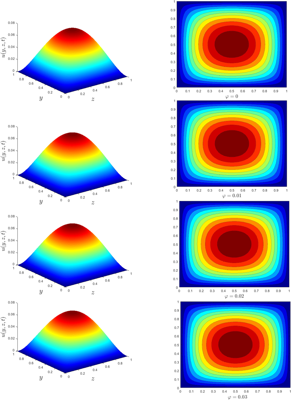
Velocity profile for different values of nanoparticle volume fraction
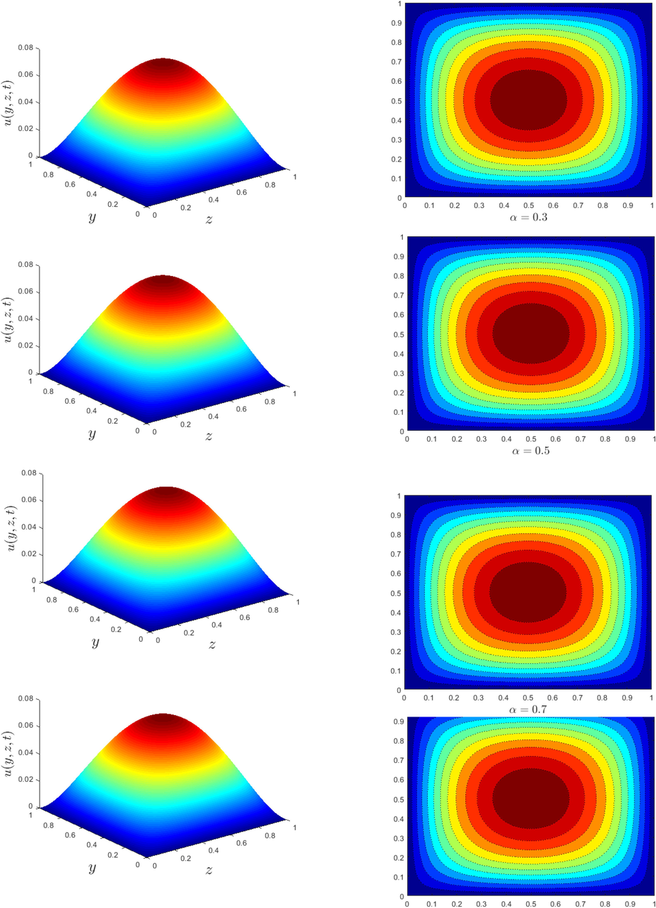
Velocity profile for different values of fractional derivative parameter
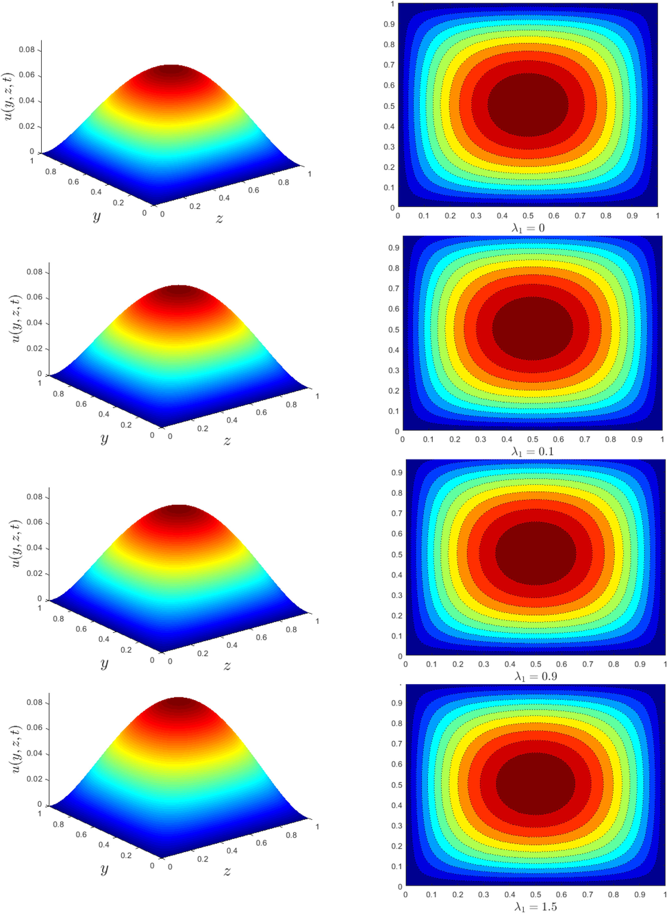
Velocity profile for different values of relaxation time
Temperature profile for different values of fractional derivative parameter
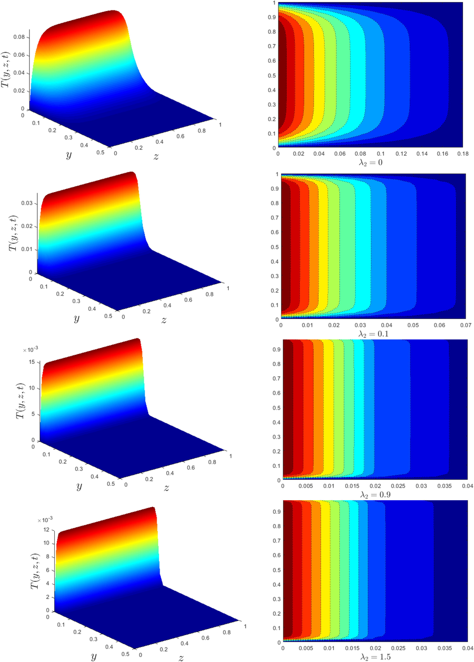
Temperature profile for different values of relaxation time
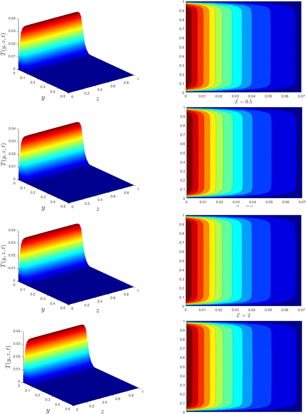
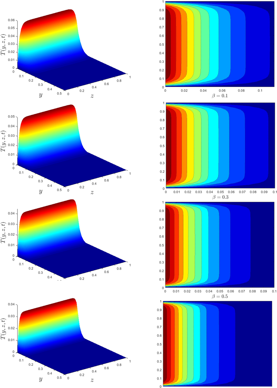
Temperature profile for different values of dissipation parameter
.
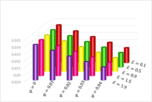
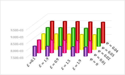
Impact of dissipation parameter
and nanomaterial volume fraction
on
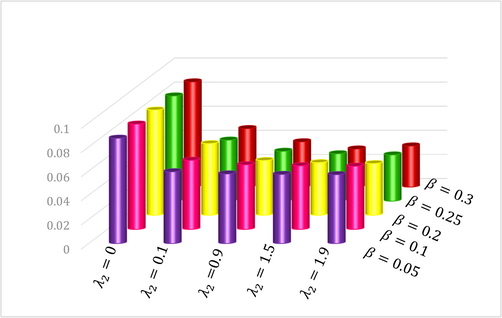
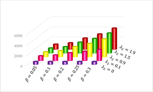
Impact of fractional parameter
and relaxation time
on
Impact of dissipation parameter
and nanomaterial volume fraction
on
Impact of fractional parameter
and relaxation time
on
To begin, the numerical computations illustrated in Fig. 1 are performed to determine the impact of the nanomaterial volume fraction on the velocity field. This figure evidenced a decrement in fluid flow velocity upon adding nanomaterials. The fluid becomes more dense as the concentration of particles inside the fluid increases, which causes a drop in velocity flow.
Fig. 2 shows features of the fractional derivative parameter on the velocity field. The fractional derivative not only quantifies the frequency-dependent complex modulus but also anticipates the relaxation and creep-responses of viscoelastic fluid (Zhao, 2020). The velocity field declines when increases. One may anticipate, that as increases, the resistance of the material particles increases which decreases the flow speed. Fig. 3 depicts the consequences of the relaxation time parameter on the velocity profile of the fluid. According to Fig. 3, the higher the relaxation time parameter, the higher the fluid velocity. The length of time needed to return to normal condition grows as increases, which increases the velocity field.
The fluctuation in the non-dimensional temperature with different values of the fractional derivative parameter can be observed in Fig. 4. The fractional derivative parameter might be a new indicator of heat conduction in a conducting material. An appropriate value of can increase the effectiveness of a thermo-electric material figure-of-merit (Ezzat, 2011). The temperature profile diminishes as increases. Increasing the magnitude of can obstruct the temperature distribution. Drawing Fig. 5 is an effort to conjure up the relation between temperature and relaxation time parameter . This resolves the paradox of unbounded heat propagation speed in thermo-electric fluid (Ezzat, 2010). The temperature profile diminishes as the value of rises. Fig. 6 shows the relationship between the viscous dissipation and the temperature of Maxwell hybrid nanofluid. As rises, the fluid’s capacity to retain heat energy increases due to friction forces, improving the temperature profile.
Next, the effects of various embedded elements on the surface temperature are sketched out in Figs. 7 and 8. The fluid temperature on the surface of the plate decreases for high volume concentration, see Fig. 7. Generally, the increased volume of nanomaterials improves the thermal conductivity of a fluid. However, several factors affect a fluid’s thermal conductivity, including the nanomaterials concentration, compatibility, preparation process, type, shape, and composition of the nanoparticles. On the other hand, the wall temperature increases due to the viscous dissipation effect. Fig. 8 shows that the surface temperature is a decreasing function of fractional derivative and relaxation time parameters.
Finally, we arrived at column graphs illustrated in Figs. 9 and 10 at this point, which depict the variation of the Nusselt number in response to various pertinent parameters. It can be seen in Fig. 9 that the maximum Nusselt number is owned by increasing nanomaterial volume concentration. It is close to physical expectations as the thermal conductivity of the fluid increases on interacting with nanomaterials. Moreover, the Nusselt number decreases abruptly for increasing values of the viscous dissipation parameter. Drawing Fig. 10 is an effort to conjure up the influences of fractional derivative and relaxation time parameter on the Nusselt number. It is observed that the Nusselt number is an increasing function of fractional derivative and relaxation time parameters.
5 Conclusions
This research is conducted to evaluate the MWCNTs-Al2O3 nanomaterials, viscous dissipation, fractional derivatives, and their impact on the flow and heat transfer characteristics of Maxwell nanofluid. The fractional UCM model is solved using the Caputo derivative and the Crank-Nicolson method. Below is a list of the main affirmative aspects:
-
The less the nanomaterial volume concentration and fractional derivative parameter, the more the velocity of Maxwell hybrid nanofluid.
-
To manifest a surface heat increase, the nanomaterial concentration, the fractional derivative parameter, and the relaxation time parameter must all be modest.
-
At high levels of the relaxation time, fractional derivative, and nanomaterial concentration parameters, Nusselt number augmentation may be projected.
-
In general, when , it is possible to predict the Newtonian fluid flow.
Acknowledgments
The authors would like to acknowledge the Ministry of Higher Education Malaysia and Research Management Centre-UTM, Universiti Teknologi Malaysia for financial support through vote number 08G33.
Declaration of Competing Interest
The authors declare that they have no known competing financial interests or personal relationships that could have appeared to influence the work reported in this paper.
References
- Heat and mass transfer of upper convected Maxwell fluid flow with variable thermo-physical properties over a horizontal melting surface. Appl. Math.. 2015;6(08):1362.
- [Google Scholar]
- Mathematical model for thermal and entropy analysis of thermal solar collectors by using Maxwell nanofluids with slip conditions, thermal radiation and variable thermal conductivity. Open Phys.. 2018;16(1):123-136.
- [Google Scholar]
- Hybrid nanofluid flow over a stretched cylinder with the impact of homogeneous-heterogeneous reactions and Cattaneo-Christov heat flux: series solution and numerical simulation. Heat Transfer. 2021;50(4):3800-3821.
- [Google Scholar]
- Thermoelectric MHD non-Newtonian fluid with fractional derivative heat transfer. Phys. B. 2010;405(19):4188-4194.
- [Google Scholar]
- Theory of fractional order in generalized thermoelectric MHD. Appl. Math. Model.. 2011;35(10):4965-4978.
- [Google Scholar]
- Slip flow of Casson-Maxwell nanofluid confined through stretchable disks. Indian J. Phys.. 2022;96(7):2041-2209.
- [Google Scholar]
- Cattaneo–Friedrich and Crank-Nicolson analysis of upper-convected Maxwell fluid along a vertical plate. Chaos, Solitons Fractals. 2021;153:111463.
- [Google Scholar]
- A finite difference method to analyze heat and mass transfer in kerosene based γ-oxide nanofluid for cooling applications. Phys. Scr.. 2021;96:095215.
- [CrossRef] [Google Scholar]
- A computational approach for boundary layer flow and heat transfer of fractional Maxwell fluid. Math. Comput. Simul. 2022;191:1-13.
- [Google Scholar]
- MHD natural convection in cadmium telluride nanofluid over a vertical cone embedded in a porous Medium. Phys. Scr.. 2019;94(12):125208.
- [Google Scholar]
- Heat transfer in cadmium telluride-water nanofluid over a vertical cone under the effects of magnetic field inside porous medium. Processes. 2019;8(1):7.
- [Google Scholar]
- A novel study on time-dependent viscosity model of magneto-hybrid nanofluid flow over a permeable cone: applications in material engineering. Eur. Phys. J. Plus. 2020;135(9):730.
- [Google Scholar]
- A novel study on hybrid model of radiative Cu–Fe3O4/water nanofluid over a cone with PHF/PWT. Eur. Phys. J. Spec. Top.. 2021;230(5):1257-1271.
- [Google Scholar]
- Applications of Fractional Calculus in Physics. World Scientific; 2000.
- Numerical investigation of MHD impact on Maxwell nanofluid. Int. Commun. Heat Mass Transfer. 2021;120:104973.
- [Google Scholar]
- Thermal characterization of coolant Maxwell type nanofluid flowing in parabolic trough solar collector (PTSC) used inside solar powered ship application. Coatings. 2021;11:1552.
- [CrossRef] [Google Scholar]
- Marangoni convective flow of hybrid nanofluid (MnZnFe2O4-NiZnFe2O4-H2O) with Darcy Forchheimer medium. Ain Shams Eng. J.. 2021;12(4):3931-4398.
- [Google Scholar]
- Dynamics of aluminum oxide and copper hybrid nanofluid in nonlinear mixed Marangoni convective flow with entropy generation: applications to renewable energy. Chin. J. Phys.. 2021;73:275-287.
- [Google Scholar]
- Rheology: Principles, Measurements and Applications. New York: Wiley-VCH; 1994.
- Numerical simulation of AA7072-AA7075/water-based hybrid nanofluid flow over a curved stretching sheet with Newtonian heating: a non-Fourier heat flux model approach. J. Mol. Liq.. 2021;335:116103.
- [Google Scholar]
- Fractional calculus in viscoelasticity: an experimental study. Commun. Nonlinear Sci. Numer. Simul.. 2010;15(4):939-945.
- [Google Scholar]
- Non-Newtonian hybrid nanofluid flow over vertically upward/downward moving rotating disk in a Darcy-Forchheimer porous medium. Eur. Phys. J. Spec. Top.. 2021;230(5):1227-1237.
- [Google Scholar]
- Parveen, Khadeeja, Viktoria Banse, and Lalita Ledwani. 2016. “Green Synthesis of Nanoparticles: Their Advantages and Disadvantages.” In AIP Conference Proceedings, 1724:020048. 1. AIP Publishing LLC.
- Numerical treatment of 2D-magneto double-diffusive convection flow of a Maxwell nanofluid: heat transport case study. Case Stud. Therm. Eng.. 2021;28:101383.
- [Google Scholar]
- Two-phase Darcy-Forchheimer flow of dusty hybrid nanofluid with viscous dissipation over a cylinder. Int. J. Appl. Comput. Math.. 2021;7(3):1-18.
- [Google Scholar]
- Thermal radiative mixed convection flow of MHD Maxwell nanofluid: implementation of Buongiorno’s model. Chin. J. Phys.. 2022;77:1465-1478.
- [Google Scholar]
- A review on performance and environmental effects of conventional and nanofluid-based thermal photovoltaics. Renew. Sustain. Energy Rev.. 2018;94:302-316.
- [Google Scholar]
- Hybrid nanofluid flow and heat transfer over backward and forward steps: a review. Powder Technol.. 2020;363:448-472.
- [Google Scholar]
- Analytical solutions and numerical schemes of certain generalized fractional diffusion models. Eur. Phys. J. Plus. 2019;134(5):199.
- [Google Scholar]
- Second-grade fluid model with Caputo-Liouville generalized fractional derivative. Chaos, Solitons Fractals. 2020;133:109631
- [Google Scholar]
- A new collection of real world applications of fractional calculus in science and engineering. Commun. Nonlinear Sci. Numer. Simul.. 2018;64:213-231.
- [Google Scholar]
- Experimental studies of nanofluid thermal conductivity enhancement and applications: A review. Renew. Sustain. Energy Rev.. 2017;75:1239-1253.
- [Google Scholar]
- New polypyrrole-multiwall carbon nanotubes hybrid materials. J. Optoelectron. Adv. Mater.. 2006;8(2):643-667.
- [Google Scholar]
- Two-phase flow of dusty fluid with suspended hybrid nanoparticles over a stretching cylinder with modified fourier heat flux. SN Appl. Sci.. 2021;3(3):1-9.
- [Google Scholar]
- Comparative analysis of (zinc ferrite, nickel zinc ferrite) hybrid nanofluids slip flow with entropy generation. Mod. Phys. Lett. B. 2021;35(20):2150342.
- [Google Scholar]
- Constitutive equation with fractional derivatives for the generalized UCM model. J. Nonnewton. Fluid Mech.. 2010;165(3–4):88-97.
- [Google Scholar]
- Axisymmetric convection flow of fractional maxwell fluid past a vertical cylinder with velocity slip and temperature jump. Chin. J. Phys.. 2020;67:501-511.
- [Google Scholar]
Appendix A
Supplementary data
Supplementary data to this article can be found online at https://doi.org/10.1016/j.jksus.2022.102389.
Appendix A
Supplementary data
The following are the Supplementary data to this article:


