Characterization and modeling of a new magnetorheological damper with meandering type valve using neuro-fuzzy

1 Introduction

Magnetorheological (MR) fluids have been used in many applications due to its sensitive rheological properties to magnetic field. MR dampers, as one of the most discussed applications of MR fluid, are one of the examples that have been proven effective in providing smart solution for vibration problems (Lam et al., 2010; Zhu et al., 2012). The ranges of MR damper applications that have been investigated are including vehicle primary suspension system, seat suspension, weapon recoil absorber, and seismic vibration isolation (Imaduddin et al., 2013; Choi et al., 2016). The application of MR damper is normally viewed in the perspective of a semi-active device. A semi-active device provides improvement to a passive device through adaptive characteristics adjustment (Choi et al., 2008; Dong et al., Jul 2009; Wang et al., 2009; Nugroho et al., 2014). A slightly different approach if compared with the active device which directly intervene the system with additional force and energy from external force. The results are that the semi-active device tends to be more efficient and affordable than the active device though with narrower range of performance improvement (Fischer and Isermann, 2004).

Like any dampers, an MR damper works by converting the kinetic energy of the fluids that flow interchangeably between chambers into heat (Dogruoz et al., 2003). The conversion occurs through a component that creates pressure loss known as the MR valve. Since the amount of pressure loss is directly corresponding to the energy converted into heat and the reaction force generated by the damper, the MR valve can be considered as the key component that determines the performance of the MR damper (Bai et al., 2013). In order to improve the damper performance, many types of valve have been developed (Abd Fatah et al., 2015). The recent development of MR valve has introduced the new generation of compact high performance MR valve as a result of the utilization of meandering flow path pattern inside the valve (Imaduddin et al., 2014; Imaduddin et al., 2015). The meandering type MR valve is utilizing the combination of multiple annular and radial flow channels which maximizes the effective area. The effective area is the term that defines the area where the magnetic flux perpendicularly encounters the MR fluid flow. The successful concept development of meandering type MR valve has been extended by many other MR valve variations such as the modular type MR valve (Ichwan et al., 2016) and the meandering flux path type MR valve (Abd Fatah et al., 2016). The meandering type MR valve is potential for many MR based applications, especially for the application that requires large energy dissipation in a compact form.

Aside from the valve design, the modeling of hysteresis phenomenon in an MR damper is also a challenging problem that has been discussed by many researchers (Choi et al., 2001; Jimenez et al., 2005; Kwok et al., 2006, 2007; Ikhouane et al., 2007; Dominguez et al., 2008, 2014; Metered et al., 2010; Sahin et al., 2010; Ubaidillah et al., 2011; Wang et al., 2011; Jiang et al., 2012; Yang et al., 2013). Hysteresis is the result of memory effect in the force restoring mechanism which depends not just on the instantaneous disturbances, but also on the previous state of disturbances. In general, the hysteresis modeling in an MR damper can be divided into two different approaches, the parametric and non-parametric approach. The parametric approach is the modeling approach that characterize the damper with combinations of several idealized physical elements such as springs and dampers. Since the assumption is set from the early stage of the modeling process, the parametric approach is normally represented in a more generic form of equation with fixed number of parameters which can be adjusted to model many types of dampers by tuning the parameters values. The known method in parametric approach are the Bouc-Wen model (Ikhouane et al., 2007; Kwok et al., 2007; Bai et al., 2015), Dahl model (Beskhyroun et al., 2012; Zhu et al., 2014), LuGre model (Jimenez et al., 2005; Imaduddin et al., 2016) and Sigmoid model (Wang et al., 2011). The non-parametric approach models the dynamics of the damper by employing analytical expressions rather than assuming a physical element like the one in parametric approach. Although the approach will not produce a generic set of equations, many studies have revealed that the non-parametric models are generally more accurate and robust than the parametric models (Wang et al., 2011). Many types of model lies in this category such as the polynomial model (Choi et al., 2001; Ubaidillah et al., 2011; Imaduddin et al., 2016), Neural Network model (Xia, 2003; Tudón-Martínez et al., 2012; Bhowmik et al., 2013), and the Neuro-Fuzzy model (Gu and Oyadiji, 2008; Wang, 2009; Nguyen and Choi, 2012; Zong et al., 2012; Zeinali et al., 2013).

The recent development of meandering type valve has opened a new opportunity to create an MR damper with higher performance capability. However, the utilization of a new valve design is also potentially changing the damping characteristics, including the hysteresis pattern. Since the valve is recently developed, the discussion about the hysteresis characteristics and modeling of the damper utilizing the valve, so far, has not been conducted. In this paper, the modeling of hysteresis phenomenon in an MR damper with the meandering type valve is presented. The hysteresis behavior is captured by measuring the damping force characteristics against harmonic excitation from the dynamic test platform. The measurement data are then modeled using neuro-fuzzy approach by dividing the data into two parts. The first part is used for training the neuro-fuzzy system while the second part is used to validate the model output. As a benchmark, the results are compared with the results from the modified LuGre model. The main contribution of this work is in the characterization of the new type MR damper using meandering type valve and its hysteresis modeling using neuro-fuzzy approach. The rest of this paper is organized as follows. Section 2 explains the conception of the bypass MR damper with the meandering type valve. The prototype preparation and the experimental setup as well as the damping characterization results are described in Section 3. Section 4 elaborates the neuro-fuzzy modeling approach for the problem including the consideration of parameter selections. The discussion of model performance including the validation, benchmarking and error analysis are given in Section 5 while the Section 6 concludes the paper.

2 MR damper with meandering type valve

The MR damper discussed in this paper is the bypass type MR damper with meandering type valve. The schematic of the MR damper is depicted in Fig. 1. According to the figure, the bypass damper components can be divided into two parts, the column section and the bypass section. The column section consists of the main cylinder, the piston and the rods while the bypass section consists of the conduit and the valve. When the piston is moving, the compressed fluid in the cylinder will be pushed to the other chamber via the bypass section pass-through the valve. The valve obstructs the flow movement and creates pressure differences between these chambers which further produce the damping force. Therefore, the variation of the obstruction, which in the case of MR valve is generated from the variation of magnetically-generated shear stress of the fluid, will result in the variation of damping force of the damper.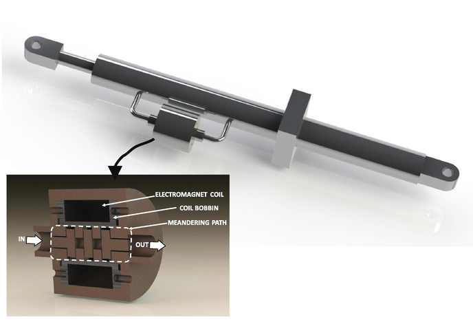

Close

Fig. 1

The illustration of bypass MR damper concept with meandering type valve.

Export to PPT

Unlike the common MR damper, which integrates the valve into the piston part, the bypass type MR damper relocates the valve outside the cylinder (Cook et al., 2007). Although the bypass configuration is obviously bulkier than the internal valve configuration, the relocation of the valve outside the column section have promised several benefits. The main benefit of the bypass configuration is the freedom of valve selection and installation since the size of the valve is not constrained by the cylinder size and length. Therefore, the synchronization of the cylinder size and valve size are irrelevant as with the same cylinder, variety selection of valves can be chosen and various damping performance ranges can be acquired. Another benefit is the ease of installation and modification since the valve can be changed easier without having to disintegrate the cylinder part.

The MR valve in the bypass section has embedded electromagnet which the flux is designed to crossed the flow path of the MR fluid. The induced magnetic field to the MR fluid rapidly changes the state of the fluid from Newtonian to Non-Newtonian form. The adjustment of magnetic flux density at the intersections regulates the yield stress of the fluid, generates pressure difference between the valve inlet and outlet and controls the fluid flow. The intersection area between the flux and fluid, which known as the effective area, is very critical since the regulation pressure drop can only be done in this area. The common practices to arrange the optimum effective area are normally divided into two types, the annular and radial valve arrangement. Both have their own benefits and limitations, however the recent progress has arrived in the combinations of these arrangements and the highest pressure drop so far can be achieved with the use of multiple combination of annular and radial valve known as the meandering flow path arrangement. The concept of meandering flow path arrangement basically aims to maximize the effective area so that the higher pressure drop controllable range and capacity can be achieved in smaller valve size. With such valve performance, higher damping controllable range of force is expected to be achieved in smaller damper size. The detail explanations about the meandering type MR valve has been discussed in Imaduddin et al. (2014, 2015).

3 Damping characterization

3.1

3.1 Experimental set up

The experimental arrangement for the damping characterization is depicted in Fig. 2. The bypass MR damper in this study is prepared with a double rod cylinder with bore size of 30 mm, rod size of 18 mm and stroke length of 70 mm. Since the piston is sealed, fluid ports are given in each end of the cylinder for connection with the bypass channel. In the middle of the bypass channel, the meandering type MR valve is installed. The meandering type MR valve used in this study is designed and manufactured by Vehicle System Engineering Research Lab. (Imaduddin et al., 2014) with both 0.5 mm annular and radial gap size. According to the design specifications, the valve with both 0.5 mm annular and radial gap configuration is able to achieve maximum pressure drop of 6.8 MPa at 1A current input to the electromagnet at around 40 ml/s of flow rate. The MR fluid filled in the damper for this study is the MRF-132DG made by Lord Corporation. The magnetic and yield stress characteristics of the MRF-132DG is depicted in Figs. 3 and 4 respectively.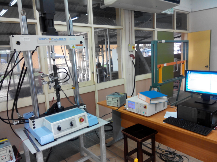

Close

Fig. 2

Experimental set up.

Export to PPT

Close

Fig. 3

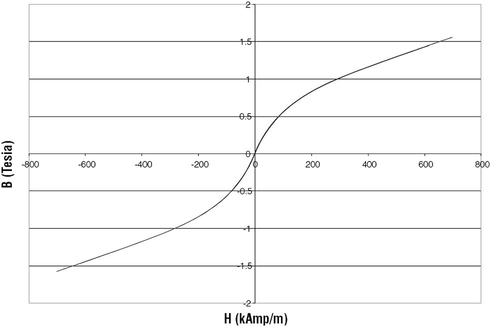
Magnetic characteristics of MRF-132DG (Lord Corp., 2011).

Export to PPT

Close

Fig. 4

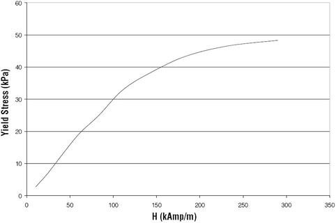
Yield stress characteristics of MRF-132DG (Lord Corp., 2011).

Export to PPT

The damping characterization is conducted by exciting the damper with sinusoidal wave generated from the hydraulically actuated Shimadzu Fatigue Dynamic Machine. The sinusoidal excitation is controlled to a fixed displacement setting of ±25 mm with frequency varied from 0.5 to 1.5 Hz. It means, the peak velocities will be varied from 78.5 mm/s to 235.6 mm/s. The damping response is measured by 20 kN capacity load cell to measure the damping force and the 100 mm displacement sensor to measure the real time excitation movement. The variation of current input to the valve electromagnet is made with the interval of 0.1 A starting from 0 to 0.8 A. To ensure data consistency, each measurement is conducted for 25 cycles of sinusoidal movement.

3.2

3.2 Damping characteristics

3.2.1

3.2.1 Frequency variation effects

The relationship between force and displacement as the primary measurement data for the off-state (no-current) condition at various frequency excitations is shown in Fig. 5. The results are taken from the 10th cycle and shows typical measurement results that are consistent for all the measurement after the 3rd cycle. According to the figure, the force constantly increases with increasing frequency. Unfortunately, the increasing of force due to the effect of frequency variations cannot be clearly visualized using the force-displacement relationship because the changing of frequency is not reflected in the displacement measurement data. If the sinusoidal displacement is expressed in the form of $u=A\cos \left(2\pi \mathit{ft}\right)$ , where Ais the excitation amplitude of the displacement and fthe frequency of excitation, the changing of frequency excitation will not have effect to the amplitude of the displacement.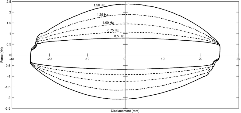

Close

Fig. 5

Off-state force-displacement characteristics at various frequency excitations.

Export to PPT

In order to visualize the effect of frequency excitation clearer, the damping characteristics should be depicted using force-velocity relationship. The velocity is not primarily measured but can be obtained using first-order differentiation of the displacement data as $\dot{u}=-A2\pi f\cos \left(2\pi \mathit{ft}\right)$ . From the equation it can be seen that the changing of frequency will have direct effect on the amplitude of the velocity. The secondary relationship between force and velocity for the off-state condition at various frequency excitations is shown in Fig. 6. According to the Figure as the frequency is increased the peak velocity is also increased in line with the peak force value. The width of the hysteresis is also changing proportional to the magnitude of peak velocity. The nonlinearity between force and velocity is also appeared in the force–velocity curve and tends to larger in the higher frequency.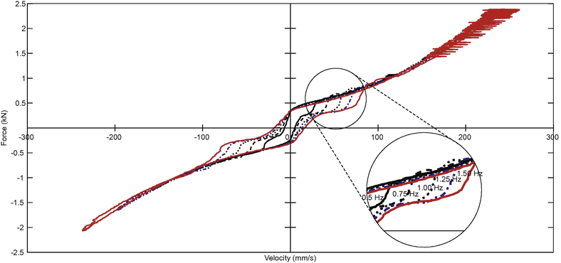

Close

Fig. 6

Off-state force-velocity characteristics at various frequency excitations.

Export to PPT

3.2.2

3.2.2 Current variation effects

The relationship between force-displacement and force-velocity for the current input varying from 0 to 0.8 A at the frequency excitation of 0.5 Hz are shown in Figs. 7 and 8 respectively. According to the figures, the force is constantly increasing when the current input is increased as a result of pressure drop increase in the valve. The average increment of damping force is around 0.65 kN for every 0.2 A raise with peak damping force of nearly 3.2 kN at 0.8 A of current input and MR effect, defines as the ratio between the on-state and the off-state, of around 4.5. It also means the achievable damping force of 0.8 A at 0.5 Hz frequency excitation is higher than the damping force of 0.0 A at 1.5 Hz frequency excitation.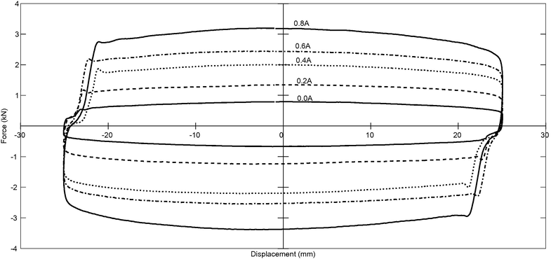

Close

Fig. 7

Influence of various current inputs to the force-displacement characteristics at 0.50 Hz excitation.

Export to PPT

Close

Fig. 8

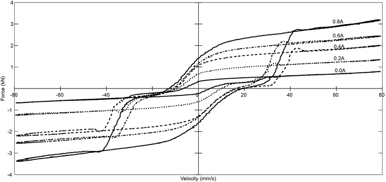
Influence of various current inputs to the force-velocity characteristics at 0.50 Hz excitation.

Export to PPT

The limitation of force-displacement curve in visualizing the damping characteristics also can be stressed with the results since the distinction between the force augmentation due to frequency excitation and the force amplification due to change of current input cannot be clearly seen at the force-displacement curve. Theoretically, it is also generally accepted that the damping effect as the form of energy dissipation is relative to the applied velocity to the damper and not displacement length. However, due to the inevitable hysteresis effect of the force-velocity characteristics, the modeling approach will normally involve the displacement data as one of the model input to make a clear distinction between the upper and lower force-velocity curve.

4 Neuro-fuzzy hysteresis model

The hysteresis phenomenon in the damping characteristics is a challenging task to model. The common approach to model the hysteresis phenomenon generally can be divided into two types, the parametric and non-parametric approach (Sahin et al., 2010; Wang et al., 2011). Each approach has its own benefit, but in terms of accuracy, the non-parametric approach is generally accepted as the more accurate approach. One of the popular method in the non-parametric approach is the Adaptive Neuro-Fuzzy Inference System (ANFIS) (Wang, 2009; Zong et al., 2012; Nguyen and Choi, 2012; Zeinali et al., 2013). ANFIS combines the fuzzy system and artificial neural network algorithm to mimic nonlinear behavior. There are 5 layers in ANFIS that aims to minimize the sum of squared error (SSE) between the desired and actual output. The first layer is the input layer, the second and third layer are the rule layers, while the fourth and fifth layer are the output layer and the summation layer respectively. The generic structure of the ANFIS is illustrated in Fig. 9.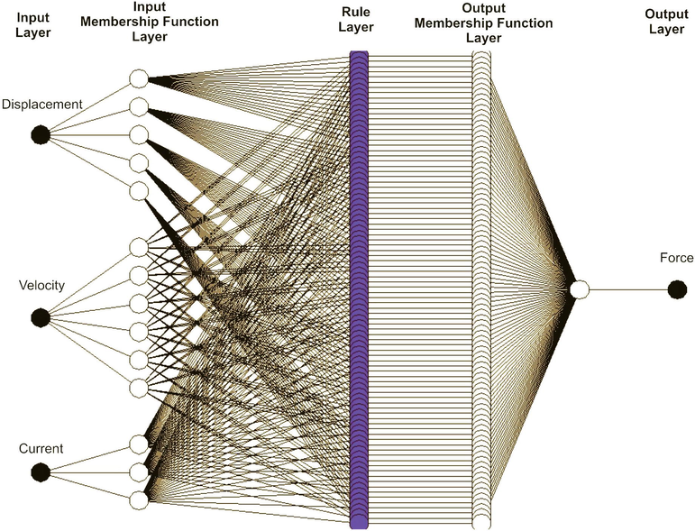

Close

Fig. 9

ANFIS structure.

Export to PPT

In the first layer, the displacement, velocity and current as the inputs of the ANFIS are defined and the Membership Functions (MF) of these inputs are initiated. At the beginning, the number of MF as well as its parameters, known as the premise parameters, for each input should be selected, however, after the training process started, the premise parameters will be adjusted. In this paper the MF function of each input is defined as Gaussian as represented in the following equation:

In the second layer, the AND-rule is implemented to express the so-called firing strength which multiplies the combination of outputs from each MF from the first layer. The output of the second layer can be expressed as follows:

In the third layer the output of each firing strength is divided by the sum of all firing strength expressed in the following equation:

The fourth layer implements the Takagi-Sugenos if-then rule where the output of the third layer is combined with the coefficient of $p_i$ , $q_i$ , $r_i$ and $s_i$ known as the consequent parameters. The outcome of each node in the fourth layer is expressed in the following:

Finally, the fifth layer provides the output of the ANFIS by computing the summation of all node output from the fourth layer in the Eq. 5:

In this paper, the MFs for displacement input, velocity input and current input are set as Gaussian shaped with 5-6-3 configuration based on the analysis of MF selection conducted by Zeinali et al. (2013), which produces 90 If-then rules. The training input of the ANFIS is based on the 10th cycle damping characteristics data from the combination of frequency excitation of 0.50 Hz to 1.50 Hz and current of 0 to 0.8 A with 0.1 A increments. The training process for ANFIS are conducted for 3500 epochs to adjust the premise and consequent parameters. Fig. 10 shows the trend of Root Mean Square Error (RMSE) for the training process while Tables 1 and 2 list the premise parameters and consequents as the results of training respectively.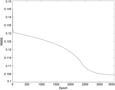

Close

Fig. 10

The trend of RMSE for 3500 epoch.

Export to PPT

5 Performance evaluation and discussions

The performance of the neuro-fuzzy hysteresis model is evaluated by comparing the output of the FIS with the measured damping characteristics. The model performance is evaluated for both variations of frequency excitation and current input. As a benchmark, the model output is also compared with the output from the recently developed parametric hysteresis model based on LuGre operator (Imaduddin et al., 2016). Since the benchmark model was originally developed for MR valve, slight modifications on input and output variable definition are needed. After modification, the modified LuGre model for MR damper proposed in this study is expressed as:

The identification process for these parameters are conducted using Parameter Estimation Toolbox in MATLAB with Gradient Descent as the optimization method. The estimation are performed using the sampling data in 1.00 Hz for each corresponding current input. The trend of each estimated parameters are then approximated using third order polynomial approximation function to current input (i) shown in Table 3.

The measured characteristics that are used for the evaluation are based on the 20th cycle measurement for 0.50 Hz, 0.75 Hz, 1.00 Hz, 1.25 Hz and 1.50 Hz. The evaluation is conducted by matching the force-velocity curve of the model output and the measured characteristics and also evaluating the relative error (RE) of the model using the following equation:

The graphical evaluations of the model performance are depicted in Fig. 11a to e. In general, it can be concluded that the model is able to match the force characteristic well especially in the post-yield regions. The agreement also generally better than the benchmark model since the deviation can be maintained in various frequency excitation is increased. The benchmarked model have the tendency to be less accurate when in the lower frequency excitation like in the case of 0.50 Hz and 0.75 Hz shown in Fig. 11a and b.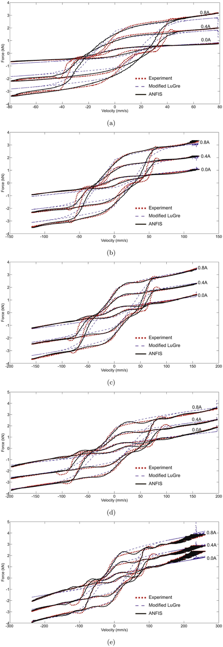

Close

Fig. 11

Validation results of the model for various current inputs and frequency excitations, (a) 0.50 Hz (b) 0.75 Hz (c) 1.00 Hz (d) 1.25 Hz (e) 1.50 Hz.

Export to PPT

There are indeed some discrepancies in the hysteresis region especially when the air-pocket effect is appeared. The occurrence of the air pocket effect is inconsistent and highly nonlinear and therefore difficult to be modeled accurately (Yun et al., 2010; Imaduddin et al., 2016). Nevertheless, according to the graphical evaluation results, both model apparently unable to replicate the air pocket effect in lower frequency excitation. However, the ANFIS model is able to show clearer air pocket effect when the frequency excitation gets higher.

The evaluation of relative error values is shown in Table 4. Overall, the results of ANFIS is clearly indicating better agreement than the modified LuGre model since, in most cases, the relative error are less than 10%. Meanwhile, the results of the modified LuGre model are only capable to produce output with relative error in around 15% limit. These results are similar with the ones reported in Imaduddin et al. (2016). Considering that the modified LuGre model is only estimated with the 1.00 Hz data, it is understandable that the relative error with the measurement in the other frequency is mediocre. Still, if the comparison is made head to head between the ANFIS and the modified LuGre model in 1.00 Hz, the ANFIS is clearly more superior with relative error nearly half of the ones in modified LuGre model. The output of the neuro-fuzzy model is also more adaptable and robust to the changing of both current input and velocity. The reason why ANFIS model performs better than the modified LuGre model in this study is mainly due to the way the neuro-fuzzy is trained. Unlike most of parametric model, like the modified LuGre, the neuro-fuzzy model is easier to be trained with ranges of inputs and outputs. In this study, the neuro-fuzzy has been trained with the 10th cycle data in all ranges of frequency excitations and current inputs making it has the exposure to all the combinations of inputs and outputs.

There is an interesting trend of relative error in both models where the values have the tendency to be less when the current input and frequency excitation are increased. However, when both current input and frequency excitation is lowered, the relative error of both models tend to increase. The tendency is matched with the observation of the graphs in Fig. 11a to e where the agreement is improved (indicates lower error) when the frequency excitation gets higher. Though, in the observation of relative error, the reduction of error is relatively stagnant when the frequency excitation is already above 1.00 Hz. There are currently no clear explanation of this trend. It may be just a specific anomaly coming from the experimental data, but it needs to be confirmed by repeating the same assessment with the other data from other range of inputs and perhaps also from the other types of MR dampers. Nonetheless, from the point of view of control design purpose, the robustness of the neuro-fuzzy model output is more beneficial since the random disturbances case that is often used as the case study in control system design requires the damper to respond wide range of velocity.

6 Conclusion

The characterization and neuro-fuzzy modeling of hysteresis behavior in an MR damper with meandering type valve have been discussed. The characterization results have shown that the dynamic relationship of damping force and velocity in the MR damper with meandering type valve are nonlinear and exhibit hysteresis phenomenon. The hysteresis phenomenon has been modeled using the neuro-fuzzy approach using three different inputs namely the displacement, velocity and current respectively while the damping force is defined as the output. The training has been conducted based on the 10th cycle characterization data for 3500 epochs and the RMSE was reduced to less than 0.105. Meanwhile, the assessment of the model performance was conducted by comparing the model output with the 20th cycle characterization data using both graphical analysis and relative error analysis. The benchmarking assessment also has been conducted by comparing the neuro-fuzzy model performance with the performance of the modified LuGre model in predicting the hysteresis phenomenon. The performance assessment results show that the neuro-fuzzy model demonstrates good agreement with the measurement data with maximum relative error of 12.5% and average relative error of around 7%. The neuro-fuzzy model is also showing better performance than the modified LuGre model in all cases that were sampled. The robustness showed in the prediction of force output in the neuro-fuzzy model is a good indication that it can be one of the superior model to be chosen in control design purpose.

References

- Design of magnetorheological valve using serpentine flux path method. Int. J. Appl. Electromagnet. Mech.. 2016;50(1):29-44.
- [Google Scholar]
- A review of design and modeling of magnetorheological valve. Int. J. Mod. Phys. B. 2015;29(04):1530004.
- Principle and validation of modified hysteretic models for magnetorheological dampers. Smart Mater. Struct.. 2015;24(8):085014.
- Principle, modeling, and testing of an annular-radial-duct magnetorheological damper. Sens. Actuators, A. 2013;201:302-309.
- New methodology for the application of vibration-based damage detection techniques. Struct. Control Health Monit.. 2012;19(8):632-649.
- Experimental calibration of forward and inverse neural networks for rotary type magnetorheological damper. Struct. Eng. Mech.. 2013;46(5):673-693.
- Fuzzy neural network control for vehicle stability utilizing magnetorheological suspension system. J. Intell. Mater. Syst. Struct.. 2008;20(4):457-466.
- A hysteresis model for the field-dependent damping force of a magnetorheological damper. J. Sound Vib.. 2001;245(2):375-383.
- State of the art of control schemes for smart systems featuring magneto-rheological materials. Smart Mater. Struct.. 2016;25(4):043001.
- Magnetorheological bypass damper exploiting flow through a porous channel. J. Intell. Mater. Syst. Struct.. 2007;18(12):1197-1203.
- Augmenting heat transfer from fail-safe magneto-rheological fluid dampers using fins. J. Intell. Mater. Syst. Struct.. 2003;14(2):79-86.
- Modeling and application of MR dampers in semi-adaptive structures. Comput. Struct.. 2008;86(3–5):407-415.
- Practical hysteresis model for magnetorheological dampers. J. Intell. Mater. Syst. Struct.. 2014;25(8):967-979.
- Comparative research on semi-active control strategies for magneto-rheological suspension. Nonlinear Dyn.. 2009;59(3):433-453.
- Mechatronic semi-active and active vehicle suspensions. Control Eng. Pract.. 2004;12(11):1353-1367.
- Application of MR damper in structural control using ANFIS method. Comput. Struct.. 2008;86(3–5):427-436.
- Development of a modular MR valve using meandering flow path structure. Smart Mater. Struct.. 2016;25(3):037001.
- Variation of the hysteresis loop with the BoucWen model parameters. Nonlinear Dyn.. 2007;48(4):361-380.
- A high performance magnetorheological valve with a meandering flow path. Smart Mater. Struct.. 2014;23(6):065017.
- Testing and parametric modeling of magnetorheological valve with meandering flow path. Nonlinear Dyn.. 2016;85(1):287-302.
- A design and modelling review of rotary magnetorheological damper. Mater. Des.. 2013;51:575-591.
- Design and performance analysis of a compact magnetorheological valve with multiple annular and radial gaps. J. Intell. Mater. Syst. Struct.. 2015;26(9):1038-1049.
- A fully dynamic magneto-rheological fluid damper model. Smart Mater. Struct.. 2012;21(6):065002.
- LuGre friction model for a magnetorheological damper. Struct. Control Health Monit.. 2005;12(1):91-116.
- A novel hysteretic model for magnetorheological fluid dampers and parameter identification using particle swarm optimization. Sens. Actuators, A. 2006;132(2):441-451.
- Bouc-Wen model parameter identification for a MR fluid damper using computationally efficient GA. ISA Trans.. 2007;46(2):167-179.
- A magnetorheological damper capable of force and displacement sensing. Sens. Actuators, A. 2010;158(1):51-59.
- Lord Corp., 2011. Lord Technical Data: MRF-132DG Magneto-Rheological Fluid. URL www.lord.com.
- The experimental identification of magnetorheological dampers and evaluation of their controllers. Mech. Syst. Signal Process.. 2010;24(4):976-994.
- A new neuro-fuzzy training algorithm for identifying dynamic characteristics of smart dampers. Smart Mater. Struct.. 2012;21(8):085021.
- An adaptive neuro fuzzy hybrid control strategy for a semiactive suspension with magneto rheological damper. Adv. Mech. Eng. 2014
- Comparison of some existing parametric models for magnetorheological fluid dampers. Smart Mater. Struct.. 2010;19(3):035012.
- An experimental artificial-neural-network-based modeling of magneto-rheological fluid dampers. Smart Mater. Struct.. 2012;21(8):085007.
- Modelling, characterisation and force tracking control of a magnetorheological damper under harmonic excitation. Int. J. Model. Ident. Control. 2011;13(1/2):9-21.
- Semi-active suspension systems for railway vehicles using magnetorheological dampers. Part I: system integration and modelling. Veh. Sys. Dyn.. 2009;47(11):1305-1325.
- Magnetorheological fluid dampers: a review of parametric modelling. Smart Mater. Struct.. 2011;20(2):023001.
- Modeling of magnetorheological damper using neuro-fuzzy system. Fuzzy Inf. Eng.. 2009;2:1157-1164.
- An inverse model of MR damper using optimal neural network and system identification. J. Sound Vib.. 2003;266(5):1009-1023.
- A new simple non-linear hysteretic model for MR damper and verification of seismic response reduction experiment. Eng. Struct.. 2013;52:434-445.
- A study on the efficiency improvement of a passive oil damper using an MR accumulator. J. Mech. Sci. Technol.. 2010;24(11):2297-2305.
- A phenomenological dynamic model of a magnetorheological damper using a neuro-fuzzy system. Smart Mater. Struct.. 2013;22(12):125013.
- Zhu, M., Wei, X., Jia, L., 2014. Building an inverse model of MR damper based on Dahl model. In: 17th International IEEE Conference on Intelligent Transportation Systems (ITSC). IEEE, pp. 1148–1153.
- Magnetorheological fluid dampers: a review on structure design and analysis. J. Intell. Mater. Syst. Struct.. 2012;23(8):839-873.
- Inverse neuro-fuzzy MR damper model and its application in vibration control of vehicle suspension system. Veh. Syst. Dyn.. 2012;50(7):1025-1041.