

Translate this page into:
Calibration under measurement errors
⁎Corresponding author. vishwagk@rediffmail.com (Gajendra K. Vishwakarma)
-
Received: ,
Accepted: ,
This article was originally published by Elsevier and was migrated to Scientific Scholar after the change of Publisher.
Peer review under responsibility of King Saud University.
Abstract
The calibration technique is the process of adjusting weights for the better enhancement of the estimate of the population parameters using auxiliary information. In this manuscript, we have proposed ratio and regression type calibration estimators for the population mean under both correlated and uncorrelated measurement errors. The variances of the proposed calibrated estimators to the first order approximation are obtained and compared their efficiencies. A Monte Carlo simulation study has been carried out to show the effect of measurement errors on the proposed calibrated estimators.
Keywords
Calibration estimation
Measurement errors
Monte Carlo

1 Introduction
The sample survey literature mainly comprised of estimating the population characteristics of the study variable using associated auxiliary information, the characteristics are closely related to the study variable and enhances our estimators for better efficiency. In this regard ratio, product and regression methods are good examples. This theory based on auxiliary information is further extended by using two or more than two auxiliary variables such as chain-type ratio cum regression, a linear combination of two auxiliary variables, etc. to estimate and enhance the estimator for better efficiency. These estimation procedures based on auxiliary information or merely on study variable presumed that all the data is free from error (without measurement errors). In the actual scenario, we never meet such ideality, that is the data is contaminated with or have hidden measurements error due to various kind of reasons, (see Cochran (1968) and Murthy (1967)). Measurement error is nothing, but a difference between the actual value and observed value. This can be revealed only when the measurement process is repeated or responses are compared to a gold standard (true value). There are many authors like Biemer and Stokes (1991), Shalabh (1997), Manisha and Singh (2001), Maneesha and Singh (2002), Carroll et al. (2006), Fuller (1987), Gregoire and Salas (2009) and Kumar et al. (2011) have given the estimation procedures for the population characteristics under the measurement errors. There is a different concern that measurement errors have presented in both the study and auxiliary variable are uncorrelated. When the same surveyor or researchers are collecting information on both study and auxiliary variable with the measurement errors then there may be a correlation between measurement errors on both study and auxiliary variable. This correlated measurement errors may arise due to hidden biased tendencies of the surveyor or researchers and can affect the estimators in many ways (see Shalabh and Tsai, 2017). While dealing with sample surveys, you may face a heterogeneous population then it is convenient to use stratified sampling than to simple random sampling. In stratified sampling, we divide the heterogeneous population into homogeneous strata that enhances our estimator for better efficacy than to simple random sampling. Here, the auxiliary information is used at the estimation stages in stratified sampling to estimating the population means. As an illustration of stratified sampling, you may see Vishwakarma and Singh (2012), and Tailor et al. (2014) of estimation procedure for the means in stratified sampling.
The statisticians are always keen to find out or employ some new technique for better precision of their proposed estimators. Calibration approach is one of them for the stratified random sampling which provides better precision for the estimators using calibration weight. It is the technique of adjusting weights for estimating population characteristics associated with characteristics based on auxiliary information as constraints. The calibration technique firstly was proffered by Deville and Sarndal (1992) which minimize the distance function (chi-square) associated with constraints. The calibration approach for the combined generalized linear regression estimator (GREG) also was made known by Singh et al. (1998). Similarly, in the reference of this, many authors like Singh (2001), Tracy et al. (2003), Kim et al. (2007), Singh and Arnab (2011), Singh (2012), Singh (2013), Clement and Enang (2015), Sinha et al. (2017), Rao et al. (2017), Singh et al. (2019), Alka et al. (2019) and, Garg and Pachori (2019) have proposed different calibration approach for estimating the population characteristics associated to different calibration constraints based on auxiliary information.
Consider a finite population , for estimating the population characteristics of the variable of matter y (known to sample only) associated with auxiliary variable x, which is known to the whole population. Let u* be the set of samples of size drawn without replacement from a population set with some probabilistic sampling having inclusion probability . In the support of the estimators and for the efficient estimation of the population characteristics , Deville and Sarndal (1992) firstly have proposed calibration estimator of the population characteristics , which is established as , where ’s are the calibration weights chosen to minimize their average distance from the basic design weights utilized in Horvitz-Thompson estimator and equal to . The Horvitz-Thompson estimator is as
Further, the impact of measurement errors ridden data on the statistical properties of the estimators of parameters like population mean and population variance, cannot be avoided in the estimation until proper care is not taken. For example, in a satellite launching, the let study variable be the path reading of the satellite and speed of the satellite be the auxiliary characteristics. Second, in a vaccine testing, let study variable be the efficacy of the vaccine and time given to preparing a vaccine be the auxiliary characteristics. If there are any measurement errors then in a satellite launching mission, mission may fail or in a vaccine testing, vaccine could be pestilent. Similarly, in a making or testing of destructive bombs, in a dog fight of fighter plane or in any others exterminatory elements, measurements errors can’t be ignored, because “a miss is as good as a mile”.
We have used some existing basic calibration estimation and the major disadvantages of this existing research is that it doesn’t count seriousness of the measurement errors. To tackle this seriousness or problems along with the variation of measurement errors. In this manuscript, we have explained the calibration technique under both correlated and uncorrelated measurement errors in stratified random sampling to examine the effect of measurement errors on the proposed estimators under different calibration weights. Here, we have described proposed estimators under two different calibration weights, in the first case, it reduced to ratio form and while in the second case it reduced to regression form. A simulation study is conducted to examine the properties of proposed estimators under both cases in measurement errors (correlated and uncorrelated) and without measurements errors in stratified sampling. Also, the efficiency comparisons have been given to examine the precision of the proposed estimators under measurements errors in stratified sampling using different calibration weights over unbiased estimator in stratified sampling. The effect of the measurement errors has given as percentage contribution of measurement errors (PCME). Further, this manuscript followed by as: proposed calibration estimators are given in Section 2, Section 3 consists of efficiency comparisons, Section 4 describes the compilation of simulation study, Section 5 describes the discussion and Section 6 mention the conclusions and further study.
2 Proposed ratio and regression type calibrated estimators under measurement errors
Let us consider a finite heterogeneous population of size N, partitioned into L non-overlapping strata of sizes Nh, h = 1,2, …, L, where Let be the pair of observed values instead of true pair values of the study character y and the auxiliary character x respectively of the jth unit in the hth stratum. Also, let be the pair of values on drawn from the hth stratum . It is familiar that in stratified random sampling an unbiased estimator of the population means of the variable and x are given by , and , , where , , and , are the sample mean of hth stratum of observed value and true value, and , and , are the population mean of hthstratum of the observed and true value. Let the observational errors be , which are normally distributed with mean zero and variances and respectively. Also let be the population correlation coefficient between and in hth stratum. For simplicity in exposition, assume that the variables uhj and vhj are correlated with correlation coefficient ρUhVh as (ythj, xthj) are correlated. The usual mean estimator and its variance under measurement error are given by
To obtaining the expression up to first degree of approximation, we have defined some error terms are given by as:
are such that with ,
and . Where and .
Thus, variance of the estimator up to first order of approximation is given by:
Case 1: Ratio form
The estimator based on Kim et al. (2007) for the population mean in stratified random sampling under measurement errors with new calibration weight is given as
Then we have the following theorem
A calibrated estimator for the population mean under measurement errors along with calibrated weight is given by:
By defining as Lagrange multiplier, and from Eqs. (8)–(10), we have Lagrange function as
Differentiating in Eq. (12) with respect to calibration weight and equating to equal to 0, we have
Multiplying above Eq. (13) by on both side and taking summation we have
Also, setting , we get combined ratio estimator in stratified random sampling under measurement errors as
, hence ratio form.
The variance of the estimator under measurement errors, to the first order approximation is given by:
From the Eq. (8), we have
and
From Eq. (16) we have
so, we have Eq. (21) as following
On setting in Eq. (22), we have new weight as
since, now substituting this in Eq. (20),
We have variance of the calibrated estimator as following
which proves the theorem 2.
The variance of the estimator without measurement errors, to the first order approximation is given by:
From the theorem 2, we have variance of the estimator under measurement errors as following
If there are no measurement errors then in the expression of the variance of the estimator , the coefficient of variation will be zero and the variance of the estimator will be now as following
this proves lemma1.
The variance of the estimator under measurement errors, to the first order approximation has greater variance than to variance of the estimator without measurement errors:
From the theorem 2 and lemma 1, the variance of the estimator under measurement errors in Eq. (19) can be expressed as following
That is , hence the proof of the lemma 2.
Case 2: Regression form
Again, we are considering here new estimator, and this estimator based on Sinha et al. (2017) for the population mean in stratified random sampling under measurement errors along with weight and is given by:
A calibrated estimator for the population mean under measurement errors along with calibrated weight is given by:
By defining and as Lagrange multiplier, and from Eqs. (26) to (28), we have Lagrange function as
Differentiating in Eq. (30) with respect to calibration weight and equating to equal to 0, we have
The estimator in Eq. (35) has another form is given by:
The variance of the calibrated estimator under correlated measurement errors, to the first order approximation is given by:
From the Eq. (37) and following the approach of Koyuncu and Kadilar (2014), and Salinas et al. (2019), we have variance of the estimator as
To obtaining the optimum value of for the minimum variance of the estimator , we are differentiating along with Eq. (39) with respect to equating it equal to zero, that is , we have
Putting the value of from the Eq. (40) in along with Eq. (39), we have minimum variance of the calibrated estimator ashence the proof of the theorem 4.
The variance of the estimator under uncorrelated measurement errors, to the first order approximation is given by:
From the theorem 4, we have variance of the estimator under correlated measurement errors as following
If there are uncorrelated measurement errors then in the expression of the variance of the estimator , the correlation coefficient will be zero and the variance of the estimator will be now as following
this proves lemma3.
The variance of the estimator without measurement errors, to the first order approximation is given by:
From the theorem 4, we have variance of the estimator under correlated measurement errors as following
If there are no measurement errors then in the expression of the variance of the estimator , the correlation coefficient and coefficient of variations will be zero, and the variance of the estimator will be now as following
this proves lemma3.
The expression for variance in lemma 4 of Eq. (42), is a variance of the classical linear regression under stratified sampling when there are no measurement errors. Similarly, the calibrated estimator from the Eq. (36) under measurement errors will be classical linear regression estimator under stratified sampling if there are no measurement errors. Therefore, this also shows that the variance of the estimator from the Eq. (37) will be equivalent to the variance of the estimator from the Eq. (36) under both correlated and uncorrelated measurements errors. That is
The variance of the estimator under measurement errors, to the first order approximation has greater variance than to variance of the estimator without measurement errors
From the lemma 3 and lemma 4, the variance of the estimator under measurement errors in Eq. (41) can be expressed as following
That is , hence the proof of the lemma 5.
3 Efficiency comparisons
In this section, we are giving efficiency comparisons of the calibrated estimators and over unbiased estimator under measurement errors.
iff
i.e.
Since see Kim et al. (2007). It is clear from Eq. (46) .
iff
Hence, the calibrated estimators and theoretically have shown supremacy over unbiased estimator under measurement errors.
4 Simulation study
To examine the merit of the proposed calibrated estimators under measurement errors, we have conducted Monte-Carlo simulation study (see Shalabh and Tsai 2017, ). The simulation study is conducted through using R studio. We have drawn heterogeneous strata of the sizes and with the total population . The different sizes of strata are drawn from a 4-variate multivariate normal distribution with means and covariance matrixwhere h = 1, 2, and 3 for the different strata with the details of the combination of the parameters. Which are given below as:
for all possible combination we have and the correlation coefficient for the correlated and uncorrelated measurement errors are as given following . Similarly, for heterogeneous case are given by as .
Further, we have drawn samples , and from each stratum with the total sample . The values of the means, estimated variances, relative efficiencies and percentage contribution of the measurement error are computed based on 5000 replications and are represented in the Tables 1–3 or by graphs in Figs. 1 and 2, see Appendix A. The relative efficiencies (RE) and percentage contribution of the measurement error (PCME) are defined respectively as
Note: For the convenient of the graphical representation, the estimators , and are represented by y, y1 and y2 respectively in all Figs. 1 and 2.
5 Discussion
To analyze the contribution of measurement errors, we have obtained two proposed calibration estimators and with their respective variances to the first order approximation under measurement errors. The two calibrated estimators and are stated in theorem 1 and 3, and their respective variances are stated in theorem 3 and 4. Lemma 1 and lemma 4 state the variances of the calibrated estimators and without measurement errors and in lemma 3, the variance of the calibrated estimator under uncorrelated measurement errors have shown. Lemma 2 and lemma 5 have shown that the variances of the calibrated estimators and have greater variances than to the respective same estimators under without measurement errors. Theoretically, lemma 2 and 5 have shown that there is contribution of measurement errors (correlated and uncorrelated). Also, in section 3, we have shown the supremacy of the calibrated estimators and over mean per unit estimator under measurement errors through the efficiency comparisons.
Thus, theoretically we have shown the aim of the study but for more analytical study, we have conducted a simulation study in Section 4. The results are shown in Tables 1–3 as a numerical and as a graphical in Figs. 1 and 2. We can see in the Tables 1–3, the relative efficiency of the proposed calibrated estimators and are greater than mean per unit estimator under measurement errors. Also, we have represented combination of data in Figs. 1 and 2 along with data level. The Figs. 1 and 2 represent the results with changing values of the correlation coefficient of the measurement errors. We can see from Figs. 1 and 2, the relative efficiency of the proposed calibrated estimators over mean per unit estimator have increased with the increasing values of the positive homogeneous correlation coefficient and have decreased with the increasing values of the negative homogeneous correlation coefficient of the measurement errors. Alike homogeneous correlation coefficient of the measurement errors, heterogeneous case has also shown the same pattern for the relative efficiency of the proposed calibrated estimators.
Theoretically, lemma 2 and 5 have shown that there is contribution of measurement errors (correlated and uncorrelated) and numerically, we have calculated as percentage contribution of measurement errors (PCME) through simulation study. We can see from the Tables 1 and 3 or from the Figs. 1 and 2, the PCME of the proposed calibrated estimators under measurement errors are increasing or decreasing with same pattern. In all the Tables 1–3 or in Figs. 1 and 2, we can see the PCME of the calibrated estimators are increasing with the increased variability of the measurement errors. In Tables 1, the proposed calibrated estimators have high values of PCME for all the cases of the uncorrelated measurement errors, that is the proposed estimators are highly affected by the measurement errors. Also, in heterogeneous correlated measurement errors case, the proposed estimators are highly affected by the measurement errors for all the variability cases of the measurement errors, But, for the positive correlated measurement errors cases not much affected. In Table 2, the proposed estimators are not much highly affected by measurement errors except in the case and for which the calibrated estimators have high values of PCME. While, in Table 3, the proposed estimators are highly affected by measurement errors for all possible correlation coefficient and variability of the measurement errors due to high values of the PCME.
In Figs. 1 and 2, the effect of measurement errors is represented with the changing values of the correlation coefficient of the measurement errors. We can see from Figs. 1 and 2, the PCME of the proposed estimators are decreasing with increased values of the positive correlation coefficient of the measurement errors and are increasing with increased values of the negative correlation coefficient of the measurement errors. Even, the PCME of the proposed estimators are high in the case of negative correlation coefficient of the measurement errors. This shows the proposed calibrated estimators are highly affected by the measurement errors than to all cases when the negative correlation coefficient of the measurement errors is observed.
6 Conclusions and further study
In this manuscript, we have proposed calibrated estimators in stratified sampling under both the correlated and uncorrelated measurement errors. The proposed calibrated estimators have shown superiority over usual mean estimator under all the cases of measurement errors and also when there are no measurement errors by theoretically as well as numerically. To examine the effect of measurement errors, we have calculated percentage contribution of measurement error () and we found that the of the calibrated estimators are increasing with increased variability of the measurement errors presented in both the study and auxiliary variables. Also, the of the calibrated estimators decreases with the positive increment of correlation coefficient of the measurement errors concerning to when there is no correlation in the measurement errors of the both variables. While, the of the calibrated estimators increases with the negative increment of the correlation coefficient of the measurement errors concerning to when there is no correlation in both the variables of the measurement errors. The calibrated estimators are highly affected by the measurement errors when the correlation coefficient in the measurement errors of the both variables are negative. A proper care should be taken in those cases where proposed estimators are highly affected by the measurement errors and specially for negative correlation coefficient of the measurement errors.
A further study can be done by applying different estimators on a calibration estimator having a calibration weight subject to fix single constraint (mean or variance), as in Eqs. (9) and (10) (see Kim et al. (2007), Clement (2017)). Second, by applying a calibration weight subject to many constraints (see Koyuncu and Kadilar (2014), Clement (2018) and Salinas et al. (2019)).
7 Disclosure of any funding to the study
No funding to carry this research work and APC.
Acknowledgments
Authors are hearty thankful to Editor-in-Chief Professor Omar Al-Dossary and three anonymous learned reviewers for their valuable comments which have made substantial improvement to bring the original manuscript to its present form.
Declaration of Competing Interest
The authors declare that they have no known competing financial interests or personal relationships that could have appeared to influence the work reported in this paper.
References
- Two-step calibration of design weights under two auxiliary variables in sample survey. J. Stat. Comput. Simul. 2019
- [CrossRef] [Google Scholar]
- Biemer, P., and S.L. Stokes (1991). Approaches to the modelling of measurement error; Measurement error in Surveys. Hoboken, NJ: Wiley, 485–516.
- Measurement Error in Nonlinear Models: A Modern Perspective. Boca Raton, FL: CRC Press; 2006.
- Calibration approach alternative ratio estimator for population mean in stratified sampling. Int. J. Statist. Econ.. 2015;16(1):83-93.
- [Google Scholar]
- A new ratio estimator of mean in survey sampling by calibration estimation. Elixir Int. J. Statist.. 2017;106:46461-46465.
- [Google Scholar]
- A note on calibration weightings for stratified double sampling with equal probability. Commun. Statist. Theory Methods. 2018;47(12):2835-2847.
- [Google Scholar]
- Measurement Error Models. Hoboken, NJ: John Wiley and Sons Inc; 1987.
- Use of coefficient of variation in calibration estimation of population mean in stratified sampling. Commun. Statist. Theory Methods 2019
- [CrossRef] [Google Scholar]
- Ratio estimation with measurement error in the auxiliary variate. Biometrics. 2009;65(2):590-598.
- [Google Scholar]
- Calibration approach estimators in stratified sampling. Statist. Probabil. Lett.. 2007;77:99-103.
- [Google Scholar]
- A new calibration estimator in stratified double sampling. Hacettepe J. Mathemat. Statist.. 2014;43(2):1-9.
- [Google Scholar]
- Some ratio type estimators under measurement error. World Appl. Sci. J.. 2011;14(2):272-276.
- [Google Scholar]
- Role of regression estimator involving measurement Errors. Braz. J. Probabil. Statist.. 2002;16:39-46.
- [Google Scholar]
- An estimation of population mean in the presence of measurement error. J. Indian Soc. Agric. Statist.. 2001;54(1):13-18.
- [Google Scholar]
- Sampling Theory and Methods. Calcutta: Statistical Publishing Society; 1967.
- On calibrated weights in stratified sampling. Austr. N. Z. Ind. Appl. Mathemat. J.. 2017;59:190-204.
- [Google Scholar]
- Calibrated estimators in two-stage sampling. Commun. Statist. Theory Methods. 2019;48(6):1449-1469.
- [Google Scholar]
- Ratio method of estimation in the presence of measurement errors. J. Indian Soc. Agric. Statist.. 1997;50:150-155.
- [Google Scholar]
- Ratio and product methods of estimation of population mean in the presence of correlated measurement error. Commun. Statist. Simul. Comput.. 2017;46(7):5566-5593.
- [Google Scholar]
- Estimation of variance of the general regression estimator: Higher level calibration approach. Survey methodology. 1998;24(1):41-50.
- [Google Scholar]
- Some calibration estimators for finite population mean in two-stage stratified random sampling. Commun. Statist. Theory Methods 2019
- [CrossRef] [Google Scholar]
- Singh, S. (2001). Generalized calibration approach for estimating variance in survey sampling. Annals of the Institute of Statistical Mathematics, 53, 404–417.
- Advanced sampling theory with applications. Vol II. Kluwer Academic Publishers; 2003.
- On the calibration of design weights using a displacement function. Metrika. 2012;75(1):85-107.
- [Google Scholar]
- Calibration approach estimation of mean in stratified sampling and stratified double sampling. Commun. Statist. Theory Method. 2017;46(10):4932-4942.
- [Google Scholar]
- Ratio and product type exponential estimators of population mean in double sampling for stratification. Commun. Statist. Appl. Methods. 2014;21(1):1-9.
- [Google Scholar]
- Note on calibration in stratified and double sampling. Surv. Methodol.. 2003;29:99-104.
- [Google Scholar]
- A general procedure for estimating the mean using double sampling for stratification and multi-auxiliary information. J. Statist. Plann. Inference. 2012;142(5):1252-1261.
- [Google Scholar]
Appendix A
Estimators
,
79.3
0.201
1.00
0
79.2
0.111
1.82
0
79.2
0.110
1.83
0
79.3
0.209
1.00
4.125
79.4
0.217
1.00
7.826
79.4
0.224
1.00
11.46
79.4
0.123
1.71
10.90
79.5
0.135
1.61
21.60
79.6
0.146
1.53
32.29
79.4
0.122
1.72
10.75
79.5
0.133
1.63
21.39
79.6
0.145
1.54
32.02
79.3
0.209
1.00
4.183
79.4
0.216
1.00
7.502
79.3
0.236
1.00
17.30
79.3
0.116
1.81
4.558
79.3
0.120
1.81
8.173
79.2
0.131
1.80
18.19
79.3
0.115
1.82
4.514
79.3
0.119
1.82
8.100
79.2
0.130
1.81
18.38
,
79.3
0.205
1.00
1.983
79.3
0.221
1.00
9.909
79.2
0.216
1.00
7.586
79.2
0.130
1.58
17.55
79.3
0.164
1.35
48.11
79.3
0.173
1.25
56.09
79.2
0.129
1.59
17.48
79.3
0.162
1.36
48.04
79.3
0.171
1.26
55.95
Estimators
,
79.3
0.205
1.00
2.174
79.3
0.211
1.00
4.872
79.4
0.216
1.00
7.757
79.3
0.116
1.76
5.312
79.3
0.122
1.73
10.35
79.4
0.131
1.65
18.37
79.3
0.116
1.78
5.216
79.3
0.121
1.74
10.20
79.4
0.130
1.67
18.15
,
79.3
0.206
1.00
2.659
79.4
0.212
1.00
5.617
79.4
0.228
1.00
13.49
79.3
0.114
1.81
3.224
79.3
0.118
1.81
6.262
79.2
0.126
1.81
13.88
79.3
0.113
1.82
3.161
79.3
0.117
1.82
6.166
79.2
0.125
1.82
14.04
,
79.3
0.208
1.00
3.317
79.3
0.216
1.00
7.351
79.5
0.227
1.00
13.24
79.3
0.112
1.86
1.075
79.2
0.117
1.85
5.408
79.4
0.121
1.88
9.213
79.3
0.111
1.87
1.055
79.2
0.116
1.86
5.465
79.4
0.120
1.90
9.177
Estimators
,
79.3
0.213
1.00
6.061
79.3
0.224
1.00
11.61
79.3
0.220
1.00
9.366
79.4
0.132
1.61
19.32
79.3
0.159
1.41
43.66
79.3
0.166
1.32
50.47
79.4
0.131
1.63
19.27
79.3
0.158
1.42
43.62
79.3
0.165
1.33
50.35
,
79.3
0.206
1.00
2.788
79.2
0.215
1.00
7.265
79.3
0.219
1.00
8.984
79.2
0.131
1.57
18.81
79.1
0.160
1.35
44.52
79.3
0.174
1.26
56.88
79.2
0.130
1.58
18.75
79.1
0.159
1.36
44.50
79.3
0.172
1.27
56.77
,
79.2
0.208
1.00
3.452
79.3
0.211
1.00
5.273
79.3
0.222
1.00
10.60
79.1
0.139
1.50
25.60
79.2
0.158
1.34
43.07
79.4
0.198
1.12
78.95
79.1
0.138
1.51
25.61
79.2
0.157
1.35
43.00
79.4
0.196
1.13
78.86
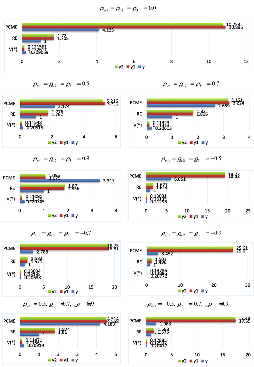
Shows variances, PCME and relative efficiencies of the calibrated estimators over usual mean estimator when .
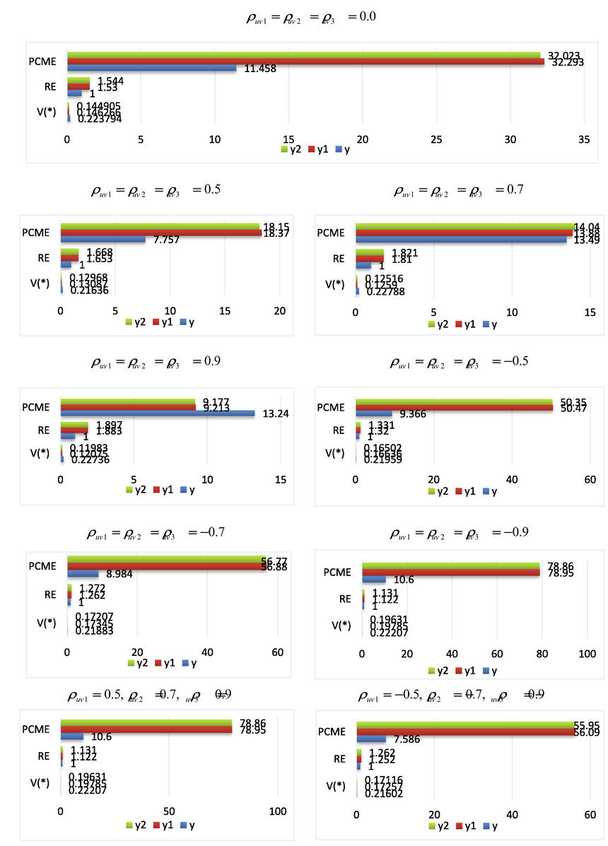
Shows variances, PCME and relative efficiencies of the calibrated estimators over usual mean estimator when .


