Approximation by Stancu variant of 


λ



-Bernstein shifted knots operators associated by Bézier basis function

Ahmed Alamer; Md. Nasiruzzaman

doi:10.1016/j.jksus.2024.103333

View/Download PDF

Buy Reprints

PDF

Translate this page into:

FulL Length Article

10 2024

:36;

103333

doi:

10.1016/j.jksus.2024.103333

Approximation by Stancu variant of $λ$ -Bernstein shifted knots operators associated by Bézier basis function

Ahmed Alamer, Md. Nasiruzzaman^⁎

Department of Mathematics, Faculty of Science, University of Tabuk, Tabuk 7149, Saudi Arabia

⁎Corresponding author. mfarooq@ut.edu.sa (Md. Nasiruzzaman) nasir3489@gmail.com (Md. Nasiruzzaman)

Received: 2024-4-8, Accepted: 2024-6-30,

Disclaimer:
This article was originally published by Elsevier and was migrated to Scientific Scholar after the change of Publisher.

Abstract

The current paper presents the $λ$ -Bernstein operators through the use of newly developed variant of Stancu-type shifted knots polynomials associated by Bézier basis functions. Initially, we design the proposed Stancu generated $λ$ -Bernstein operators by means of Bézier basis functions then investigate the local and global approximation results by using the Ditzian–Totik uniform modulus of smoothness of step weight function. Finally we establish convergence theorem for Lipschitz generated maximal continuous functions and obtain some direct theorems of Peetre’s $K$ -functional. In addition, we establish a quantitative Voronovskaja-type approximation theorem.

Keywords

41A25

41A36

33C45

Bernstein basis polynomial

Bézier basis function

λ-Bernstein-polynomial

Shifted knots

Stancu operators

Ditzian–Totik uniform modulus of smoothness

Lipschitz maximal functions

Peetre’s K-functional

Data availability

This study was not supported by any data.

1 Introduction and preliminaries

One of the most well-known mathematicians in the world, S. N. Bernstein, provided the quickest and most elegant demonstration of one of the most well-known Weierstrass approximation theorems. Bernstein also devised the series of positive linear operators implied by ${B_{s}}_{s \geq 1}$ . The famous Bernstein polynomial, defined in Bernstein (2012), was found to be a function that uniformly approximates on $[0, 1]$ for all $f \in C [0, 1]$ (the class of all continuous functions). This finding was made in Bernstein’s study. Thus, for any $y \in [0, 1]$ , the well-known Bernstein polynomial has the following results. $B_{s} (g; y) = \sum_{i = 0}^{s} g (\frac{i}{s}) b_{s, i} (y),$ where $b_{s, i} (y)$ are the Bernstein polynomials with a maximum degree of $s$ and $s \in N$ (the positive integers), which defined by

(1.1)

b_{s, i} (y) = \{\begin{matrix} (\binom{s}{i}) y^{i} {(1 - y)}^{s - i} & for s, y \in [0, 1] and i = 0, 1, \dots \\ 0 & for any i > s or i < 0 . \end{matrix}

Testing the Bernstein-polynomials’ recursive relation is not too difficult. The recursive relationship for Bernstein-polynomials $b_{s, i} (y)$ is quite simple to test. $b_{s, i} (y) = (1 - y) b_{s - 1, i} (y) + y b_{s - 1, i - 1} (y) .$

In 2010, Cai and colleagues introduced $λ \in [- 1, 1]$ is the shape parameter for the new Bézier bases, which they called $λ$ -Bernstein operators. This definition of the Bernstein-polynomials is defined as follows:

(1.2)

B_{s, λ} (g; y) = \sum_{i = 0}^{s} g (\frac{i}{s}) {\tilde{b}}_{s, i} (λ; y),

where the Bernstein polynomial

b_{s, i} (y)

expressed regarding the latest Bernstein basis function (Ye et al., 2010),

{\tilde{b}}_{s, i} (λ; y)

defined as follows by Ye et al.:

{\tilde{b}}_{s, 0} (λ; y) = b_{s, 0} (y) - \frac{λ}{s + 1} b_{s + 1, 1} (y),

{\tilde{b}}_{s, i} (λ; y) = b_{s, i} (y) + λ (\frac{s - 2 i + 1}{s^{2} - 1} b_{s + 1, i} (y) - \frac{s - 2 i - 1}{s^{2} - 1} b_{s + 1, i + 1} (y)), for i \in [1, s - 1]

{\tilde{b}}_{s, s} (λ; y) = b_{s, s} (y) - \frac{λ}{s + 1} b_{s + 1, s} (y),

where if hen

λ = 0

, then

{\tilde{b}}_{s, i} (λ; y)

reduce to classical Bernstein polynomial

b_{s, i} (y)

by (1.1). It should be noted that adding the form parameter

λ

gives us more modeling flexibility. Using shifted knots polynomials, Gadjiev and Ghorbanalizadeh (2010), introduced the Bernstein-polynomials, which include the Stancu type polynomial by:

(1.3)

S_{s, μ_{1}, μ_{2}}^{ν_{1}, ν_{2}} (g; y) = {(\frac{s + ν_{2}}{s})}^{s} \sum_{i = 0}^{s} (\binom{s}{i}) {(y - \frac{μ_{2}}{s + ν_{2}})}^{i} {(\frac{s + μ_{2}}{s + ν_{2}} - y)}^{s - i} g (\frac{i + μ_{1}}{s + ν_{1}})

where for all

i = 1, 2

the positive real numbers are

μ_{i}, ν_{i}

such that

0 \leq μ_{2} \leq μ_{1} \leq ν_{1} \leq ν_{2}

and

y \in [\frac{μ_{2}}{s + ν_{2}}, \frac{s + μ_{2}}{s + ν_{2}}]

Through approximation procedures, researchers have recently developed Bernstein type operators. Among them are the new type $λ$ -Bernstein polynomials (Aslan and Mursaleen, 2022), blending type Bernstein– Schurer–Kantorovich Operators (Ayman-Mursaleen et al., 2023), the $q$ -Bernstein–Stancu–Kantorovich operators (Ayman-Mursaleen et al., 2022), $λ$ -Bernstein operators via power series summability (Braha et al., 2020), $λ$ -Hybrid type operators (Heshamuddin et al., 2023), $α$ -Stancu–Schurer–Kantorovich operators (Heshamuddin et al., 2022), Bernstein–Kantorovich operators in Stancu variation (Mohiuddine and Özger, 2020), the Bernstein–Durrmeyer operators in Genuine modified form Mohiuddine et al. (2018), the new family of Bernstein–Kantorovich operators (Mohiuddine et al., 2017), Bézier bases with Schurer polynomials (Özger, 2020), $λ$ -Bernstein–Kantorovich operators (Rahman et al., 2019), Bernstein operators based on Bézier bases (Srivastava et al., 2019), Error estimates using Higher modulus of smoothness (Srivastava and Bisht, 2022), approximation of Bernstein type operators (Zeng and Cheng, 2001) and reference there in. Most recent in article (Ayman-Mursaleen et al., 2024), $λ$ -Bernstein-polynomial of shifted knots type operators which are associated by Bézier bases have been constructed and obtained Lemma 1.1 as follows:

(1.4)

B_{s, λ}^{ϰ_{1}, ϰ_{2}} (g; y) = {(\frac{s + ϰ_{2}}{s})}^{s} \sum_{i = 0}^{s} {\tilde{b}}_{s, i}^{ϰ_{1}, ϰ_{2}} (λ; y) g (\frac{i}{s}),

Lemma 1.1

For the test function $g (t) = 1, t, t^{2}$ , the operators $B_{s, λ}^{ϰ_{1}, ϰ_{2}}$ having: $B_{s, λ}^{ϰ_{1}, ϰ_{2}} (1; y) = 1;$ $B_{s, λ}^{ϰ_{1}, ϰ_{2}} (t; y) = \frac{1}{(s - 1) s} ((s + ν) (s - 1) - 2 λ) (y - \frac{μ}{s + ϰ_{2}}) + \frac{λ}{(s - 1) s} {(\frac{s + ϰ_{2}}{s})}^{s} [{(y - \frac{ϰ_{1}}{s + ϰ_{2}})}^{s + 1} - {(\frac{s + ϰ_{1}}{s + ϰ_{2}} - y)}^{s + 1} + {(\frac{s + ϰ_{2}}{s})}^{1 - s}];$ $B_{s, λ}^{ϰ_{1}, ϰ_{2}} (t^{2}; y) = \frac{1}{s} [{(\frac{s + ϰ_{2}}{s})}^{s} + \frac{2 λ}{s - 1}] (y - \frac{ϰ_{1}}{s + ϰ_{2}}) + \frac{1}{s^{2}} (\frac{s + ϰ_{2}}{s}) ((s + ϰ_{2}) (s - 1) - 4 λ) {(y - \frac{ϰ_{1}}{s + ϰ_{2}})}^{2} + λ {(\frac{s + ϰ_{2}}{s})}^{s} [\frac{1}{s + 1} + \frac{{(s + 1)}^{2}}{s^{2} (s - 1)}] {(y - \frac{ϰ_{1}}{s + ϰ_{2}})}^{s + 1} + \frac{λ}{s^{2} (s - 1)} {(\frac{s + ϰ_{2}}{s})}^{s} {(\frac{s + ϰ_{1}}{s + ϰ_{2}} - y)}^{s + 1} - \frac{λ}{s^{2} (s - 1)} (\frac{s + ϰ_{2}}{s}) .$

2 Operators using Bézier bases and calculating fundamental moments

Our goal in this section is to form the Stancu type of $λ$ -Bernstein shifted knots operators enhanced by Bézier bases function. Our new construction of these types operators give a valuable research path to researcher in the field of approximation theory. Researcher can use the Bézier bases function, shifted knots properties as well as Stancu type construction in various research article and explore it to get a better observation and more flexibility. For more related results and its applications we would rather have operators of the Bernstein type (Cai et al., 2018; Gadjiev and Ghorbanalizadeh, 2010; Ye et al., 2010 ). By using the shifted knots properties (see Gadjiev and Ghorbanalizadeh (2010)), we design the Bernstein basis function $b_{s, i}^{ϰ_{1}, ϰ_{2}}$ as follows:

(2.1)

b_{s, i}^{ϰ_{1}, ϰ_{2}} (y) = (\binom{s}{i}) {(y - \frac{ϰ_{1}}{s + ϰ_{2}})}^{i} {(\frac{s + ϰ_{1}}{s + ϰ_{2}} - y)}^{s - i} .

In addition, we design the Bézier bases function

{\tilde{b}}_{s, i}^{ϰ_{1}, ϰ_{2}}

by means of Bernstein basis function

b_{s, i}^{ϰ_{1}, ϰ_{2}}

(see Ye et al. (2010)) such as follows:

{\tilde{b}}_{s, 0}^{ϰ_{1}, ϰ_{2}} (λ; y) = b_{s, 0}^{ϰ_{1}, ϰ_{2}} (y) - \frac{λ}{s + 1} b_{s + 1, 1}^{ϰ_{1}, ϰ_{2}} (y),

{\tilde{b}}_{s, i}^{ϰ_{1}, ϰ_{2}} (λ; y) = b_{s, i}^{ϰ_{1}, ϰ_{2}} (y) + λ (\frac{s - 2 i + 1}{s^{2} - 1} b_{s + 1, i}^{ϰ_{1}, ϰ_{2}} (y) - \frac{s - 2 i - 1}{s^{2} - 1} b_{s + 1, i + 1}^{ϰ_{1}, ϰ_{2}} (y)), for 1 \leq i \leq s - 1

{\tilde{b}}_{s, s}^{ϰ_{1}, ϰ_{2}} (λ; y) = b_{s, s}^{ϰ_{1}, ϰ_{2}} (y) - \frac{λ}{s + 1} b_{s + 1, s}^{ϰ_{1}, ϰ_{2}} (y) .

Thus for all

\frac{ϰ_{1}}{s + ϰ_{2}} \leq y \leq \frac{s + ϰ_{1}}{s + ϰ_{2}}

and the real number

0 \leq ϰ_{1} \leq ξ_{1} \leq ξ_{2} \leq ϰ_{2}

, we define the Stancu variant of

λ

-Bernstein shifted knots operators associated by Bézier bases function

{\tilde{b}}_{s, i}^{ϰ_{1}, ϰ_{2}}

as follows:

(2.2)

S_{s, λ}^{ϰ_{1}, ϰ_{2}} (g; y) = {(\frac{s + ϰ_{2}}{s})}^{s} \sum_{i = 0}^{s} {\tilde{b}}_{s, i}^{ϰ_{1}, ϰ_{2}} (λ; y) g (\frac{i + ξ_{1}}{s + ξ_{2}}),

Remark 2.1

For operators $S_{s, λ}^{ϰ_{1}, ϰ_{2}}$ , we have the following observations:

if take $ξ_{1} = ξ_{2} = 0$ , operators $S_{s, λ}^{ϰ_{1}, ϰ_{2}}$ having the polynomials and moments raised in Ayman-Mursaleen et al. (2024) by equality (1.4);
for the choice of $ξ_{1} = ξ_{2} = 0$ and $ϰ_{1} = ϰ_{2} = 0$ , operators $S_{s, λ}^{ϰ_{1}, ϰ_{2}}$ having the polynomials and moments raised in Cai et al. (2018) by Cai et al. (2018);
for the choice of $ξ_{1} = ξ_{2} = 0$ and $ϰ_{1} = ϰ_{2} = 0$ , with $λ = 0$ , operators $S_{s, λ}^{ϰ_{1}, ϰ_{2}}$ converted to classical Bernstein operators (Bernstein, 2012);
Clearly, instead of Ayman-Mursaleen et al. (2024), Bernstein (2012) and Cai et al. (2018), we might say that our new operators are the most recent approximation results that are generalized.

This paper’s primary structure is as follows: We examine our new operators, (2.2), moments and central moments. We explore an approximation theorem of Korovkin, establish a theorem of local approximation, offer a theorem of convergence for Lipschitz maximal space and generate an asymptotic convergence results of Voronovskaja type.

Lemma 2.2

Take $g (t) = 1, t, t^{2}$ the test function, then for any $s \in {2, 3, 4, \dots .}$ , the operators $S_{s, λ}^{ϰ_{1}, ϰ_{2}}$ defined by (2.2), having the following equalities: $S_{s, λ}^{ϰ_{1}, ϰ_{2}} (1; y) = 1;$ $S_{s, λ}^{ϰ_{1}, ϰ_{2}} (t; y) = (\frac{s + ϰ_{2}}{s + ξ_{2}} - \frac{2 λ}{(s + ξ_{2}) (s - 1)}) (y - \frac{ϰ_{1}}{s + ϰ_{2}}) + \frac{λ}{(s - 1) (s + ξ_{2})} {(\frac{s + ϰ_{2}}{s})}^{s} [{(y - \frac{ϰ_{1}}{s + ϰ_{2}})}^{s + 1} - {(\frac{s + ϰ_{1}}{s + ϰ_{2}} - y)}^{s + 1}] + \frac{λ}{(s - 1) (s + ξ_{2})} (\frac{s + ϰ_{2}}{s}) + \frac{1}{(s + ξ_{2})};$ $S_{s, λ}^{ϰ_{1}, ϰ_{2}} (t^{2}; y) = \frac{s}{{(s + ξ_{2})}^{2}} [{(\frac{s + ϰ_{2}}{s})}^{s} + \frac{2 λ}{s - 1}] (y - \frac{ϰ_{1}}{s + ϰ_{2}}) + \frac{s (s + ϰ_{2})}{{(s + ξ_{2})}^{2}} [\frac{s - 1}{s} \frac{s + ϰ_{2}}{s} - \frac{4 λ}{s^{2}}] {(y - \frac{ϰ_{1}}{s + ϰ_{2}})}^{2} + λ \frac{s^{2}}{{(s + ξ_{2})}^{2}} {(\frac{s + ϰ_{2}}{s})}^{s} [\frac{1}{s + 1} + \frac{{(s + 1)}^{2}}{(s - 1) s^{2}}] {(y - \frac{ϰ_{1}}{s + ϰ_{2}})}^{s + 1} + \frac{λ}{(s - 1) {(s + ξ_{2})}^{2}} (\frac{s + ϰ_{2}}{s}) [{(\frac{s + ϰ_{2}}{s})}^{s - 1} {(\frac{s + ϰ_{1}}{s + ϰ_{2}} - y)}^{s + 1} - 1] + \frac{2 s ξ_{1}}{{(s + ξ_{2})}^{2}} (y - \frac{ϰ_{1}}{s + ϰ_{2}}) (\frac{s + ϰ_{2}}{s} - \frac{2 λ}{s (s - 1)}) + \frac{2 λ ξ_{1}}{(s - 1) {(s + ξ_{2})}^{2}} {(\frac{s + ϰ_{2}}{s})}^{s} [{(y - \frac{ϰ_{1}}{s + ϰ_{2}})}^{s + 1} - {(\frac{s + ϰ_{1}}{s + ϰ_{2}} - y)}^{s + 1}] + \frac{2 λ ξ_{1}}{(s - 1) {(s + ξ_{2})}^{2}} (\frac{s + ϰ_{2}}{s}) + \frac{1}{(s + ξ_{2})} \frac{2 s ξ_{1}}{{(s + ξ_{2})}^{2}} + \frac{ξ_{1}^{2}}{{(s + ξ_{2})}^{2}} .$

Proof

We proof the equalities as follows: $S_{s, λ}^{ϰ_{1}, ϰ_{2}} (1; y) = {(\frac{s + ϰ_{2}}{s})}^{s} \sum_{i = 0}^{s} {\tilde{b}}_{s, i}^{ϰ_{1}, ϰ_{2}} (λ; y) = B_{s, λ}^{ϰ_{1}, ϰ_{2}} (1; y) = 1;$ $S_{s, λ}^{ϰ_{1}, ϰ_{2}} (t; y) = {(\frac{s + ϰ_{2}}{s})}^{s} \sum_{i = 0}^{s} (\frac{i + ξ_{1}}{s + ξ_{2}}) {\tilde{b}}_{s, i}^{ϰ_{1}, ϰ_{2}} (λ; y) = {(\frac{s + ϰ_{2}}{s})}^{s} \sum_{i = 0}^{s} \frac{i}{(s + ξ_{2})} {\tilde{b}}_{s, i}^{ϰ_{1}, ϰ_{2}} (λ; y) + \frac{ξ_{1}}{(s + ξ_{2})} {(\frac{s + ϰ_{2}}{s})}^{s} \sum_{i = 0}^{s} {\tilde{b}}_{s, i}^{ϰ_{1}, ϰ_{2}} (λ; y) = \frac{s}{(s + ξ_{2})} {(\frac{s + ϰ_{2}}{s})}^{s} \sum_{i = 0}^{s} (\frac{i}{s}) {\tilde{b}}_{s, i}^{ϰ_{1}, ϰ_{2}} (λ; y) + \frac{ξ_{1}}{(s + ξ_{2})} B_{s, λ}^{ϰ_{1}, ϰ_{2}} (1; y) = \frac{s}{(s + ξ_{2})} B_{s, λ}^{ϰ_{1}, ϰ_{2}} (t; y) + \frac{ξ_{1}}{(s + ξ_{2})};$ $S_{s, λ}^{ϰ_{1}, ϰ_{2}} (t^{2}; y) = {(\frac{s + ϰ_{2}}{s})}^{s} \sum_{i = 0}^{s} {(\frac{i + ξ_{1}}{s + ξ_{2}})}^{2} {\tilde{b}}_{s, i}^{ϰ_{1}, ϰ_{2}} (λ; y) = {(\frac{s + ϰ_{2}}{s})}^{s} \sum_{i = 0}^{s} \frac{i^{2}}{{(s + ξ_{2})}^{2}} {\tilde{b}}_{s, i}^{ϰ_{1}, ϰ_{2}} (λ; y) + {(\frac{s + ϰ_{2}}{s})}^{s} \sum_{i = 0}^{s} \frac{2 i ξ_{1}}{{(s + ξ_{2})}^{2}} {\tilde{b}}_{s, i}^{ϰ_{1}, ϰ_{2}} (λ; y) + {(\frac{s + ϰ_{2}}{s})}^{s} \sum_{i = 0}^{s} \frac{ξ_{1}^{2}}{{(s + ξ_{2})}^{2}} {\tilde{b}}_{s, i}^{ϰ_{1}, ϰ_{2}} (λ; y) = \frac{s^{2}}{{(s + ξ_{2})}^{2}} {(\frac{s + ϰ_{2}}{s})}^{s} \sum_{i = 0}^{s} \frac{i^{2}}{s^{2}} {\tilde{b}}_{s, i}^{ϰ_{1}, ϰ_{2}} (λ; y) + \frac{2 s ξ_{1}}{{(s + ξ_{2})}^{2}} \sum_{i = 0}^{s} \frac{i}{s} {\tilde{b}}_{s, i}^{ϰ_{1}, ϰ_{2}} (λ; y) + \frac{ξ_{1}^{2}}{{(s + ξ_{2})}^{2}} \sum_{i = 0}^{s} {\tilde{b}}_{s, i}^{ϰ_{1}, ϰ_{2}} (λ; y) = \frac{s^{2}}{{(s + ξ_{2})}^{2}} B_{s, λ}^{ϰ_{1}, ϰ_{2}} (t^{2}; y) + \frac{2 s ξ_{1}}{{(s + ξ_{2})}^{2}} B_{s, λ}^{ϰ_{1}, ϰ_{2}} (t; y) + \frac{ξ_{1}^{2}}{{(s + ξ_{2})}^{2}} B_{s, λ}^{ϰ_{1}, ϰ_{2}} (1; y) .$ Thus finally, we get $S_{s, λ}^{ϰ_{1}, ϰ_{2}} (t^{2}; y)$ . □

Lemma 2.3

For the operators $S_{s, λ}^{ϰ_{1}, ϰ_{2}}$ , we get the following central moments: $S_{s, λ}^{ϰ_{1}, ϰ_{2}} (t - y; y) = (\frac{s + ϰ_{2}}{s + ξ_{2}} - \frac{2 λ}{(s + ξ_{2}) (s - 1)} - 1) y + \frac{λ}{(s - 1) (s + ξ_{2})} {(\frac{s + ϰ_{2}}{s})}^{s} [{(y - \frac{ϰ_{1}}{s + ϰ_{2}})}^{s + 1} - {(\frac{s + ϰ_{1}}{s + ϰ_{2}} - y)}^{s + 1}] + \frac{λ}{(s - 1) (s + ξ_{2})} (\frac{s + ϰ_{2}}{s}) + \frac{2 λ ϰ_{1}}{(s + ξ_{2}) (s + ϰ_{2}) (s - 1)} + \frac{1 - ϰ_{1}}{s + ξ_{2}}$ $S_{s, λ}^{ϰ_{1}, ϰ_{2}} ({(t - y)}^{2}; y) = \frac{s}{{(s + ξ_{2})}^{2}} [{(\frac{s + ϰ_{2}}{s})}^{s} + \frac{2 λ}{s - 1}] (y - \frac{ϰ_{1}}{s + ϰ_{2}}) + \frac{s (s + ϰ_{2})}{{(s + ξ_{2})}^{2}} [\frac{s - 1}{s} \frac{s + ϰ_{2}}{s} - \frac{4 λ}{s^{2}}] {(y - \frac{ϰ_{1}}{s + ϰ_{2}})}^{2} + λ \frac{s^{2}}{{(s + ξ_{2})}^{2}} {(\frac{s + ϰ_{2}}{s})}^{s} [\frac{{(s + 1)}^{2}}{(s - 1) s^{2}} + \frac{1}{s + 1}] {(y - \frac{ϰ_{1}}{s + ϰ_{2}})}^{s + 1} + \frac{λ}{(s - 1) {(s + ξ_{2})}^{2}} (\frac{s + ϰ_{2}}{s}) [{(\frac{s + ϰ_{2}}{s})}^{s - 1} {(\frac{s + ϰ_{1}}{s + ϰ_{2}} - y)}^{s + 1} - 1] + \frac{2 s ξ_{1}}{{(s + ξ_{2})}^{2}} (y - \frac{ϰ_{1}}{s + ϰ_{2}}) (\frac{s + ϰ_{2}}{s} - \frac{2 λ}{s (s - 1)}) + \frac{2 λ ξ_{1}}{(s - 1) {(s + ξ_{2})}^{2}} {(\frac{s + ϰ_{2}}{s})}^{s} [{(y - \frac{ϰ_{1}}{s + ϰ_{2}})}^{s + 1} - {(\frac{s + ϰ_{1}}{s + ϰ_{2}} - y)}^{s + 1}] + \frac{2 λ ξ_{1}}{(s - 1) {(s + ξ_{2})}^{2}} (\frac{s + ϰ_{2}}{s}) + \frac{1}{(s + ξ_{2})} \frac{2 s ξ_{1}}{{(s + ξ_{2})}^{2}} + \frac{ξ_{1}^{2}}{{(s + ξ_{2})}^{2}} + y^{2} - 2 (\frac{s + ϰ_{2}}{s + ξ_{2}} - \frac{2 λ}{(s + ξ_{2}) (s - 1)}) (y - \frac{ϰ_{1}}{s + ϰ_{2}}) y + \frac{2 λ y}{(s - 1) (s + ξ_{2})} {(\frac{s + ϰ_{2}}{s})}^{s} [{(\frac{s + ϰ_{1}}{s + ϰ_{2}} - y)}^{s + 1} - {(y - \frac{ϰ_{1}}{s + ϰ_{2}})}^{s + 1}] - \frac{2 λ y}{(s - 1) (s + ξ_{2})} (\frac{s + ϰ_{2}}{s}) - \frac{2 y}{(s + ξ_{2})} .$

3 Convergence properties of operators $S_{s, λ}^{ϰ_{1}, ϰ_{2}}$

For operators (2.2), we derive various global and local approximation theorems in this section. Using the Ditzian–Totik uniform modulus of smoothness, we first define the uniform convergence property for our operators and then obtain the local and global approximations. Next, we derive some straightforward theorems based on the Lipschitz type maximal approximation property and Peetre’s $K$ -functional property. Let we denote $W = C [0, 1]$ , the set of all continuous function on $[0, 1]$ . Given a continuous function $f$ in $W$ on $[0, 1]$ , we may replace $ℓ$ with a real-valued function equipped by norm $∥ ℓ ∥_{W} = {sup}_{y \in [0, 1]} | ℓ (y) |$ .

Theorem 3.1

Theorem 3.1 Altomare, 2010; Korovkin, 1953

Let the sequences of positive linear operators $L_{s} : C [μ_{1}, μ_{2}] \to C [μ_{1}, μ_{2}]$ for all $j = 0, 1, 2$ ${lim}_{s \to \infty} L_{s} (t^{j}; y) = y^{j}$ , is uniformly on $[μ_{1}, μ_{2}]$ . Then, for each $ℓ \in C [μ_{1}, μ_{2}]$ we get ${lim}_{s \to \infty} L_{s} (ℓ) = ℓ$ is uniformly converges for each compact subset contained in $[μ_{1}, μ_{2}]$ .

Theorem 3.2

Regarding all $ℓ \in C [0, 1]$ we get $lim_{s \to \infty} S_{s, λ}^{ϰ_{1}, ϰ_{2}} (ℓ; y) = ℓ (y)$ is converges uniformly on $[0, 1]$ .

Proof

According to Lemma 2.2, it is evident that for any $j = 0, 1, 2$ , $lim_{s \to \infty} S_{s, λ}^{ϰ_{1}, ϰ_{2}} (t^{j}; y) = y^{j},$ thus, by applying the famous Bohman–Korovkin–Popoviciu theorem, easy to get operators $S_{s, λ}^{ϰ_{1}, ϰ_{2}} (ℓ; y)$ are uniformly converge to set $ℓ \in W$ . □

Theorem 3.3

Theorem 3.3 Gadziev, 1976; Gadjiev, 1974

For the operators ${L_{s}}_{s \geq 1} : W \to W$ , let ${lim}_{s \to \infty} {‖ L_{s} (t^{β}) - y^{β} ‖}_{W} = 0, β = 0, 1, 2$ . We get for all $ℓ \in W$ , $lim_{s \to \infty} {‖ L_{s} (ℓ) - ℓ ‖}_{W} = 0 .$

Theorem 3.4

Suppose the operators $S_{s, λ}^{ϰ_{1}, ϰ_{2}} : W \to W$ , which having ${lim}_{s \to \infty} {‖ S_{s, λ}^{ϰ_{1}, ϰ_{2}} (t^{j}) - y^{j} ‖}_{W} = 0$ . For all $ℓ \in W$ we obtain $lim_{s \to \infty} ∥ S_{s, λ}^{ϰ_{1}, ϰ_{2}} (ℓ) - ℓ ∥_{W} = 0 .$

Proof

We take in account Theorem 3.3 and famous Bohman–Korovkin-Popoviciu theorem then easily we lead to show that $lim_{s \to \infty} {‖ S_{s, λ}^{ϰ_{1}, ϰ_{2}} (t^{j}) - y^{j} ‖}_{W} = 0, j = 0, 1, 2 .$ In the view of Lemma 2.2, easy to obtain ${‖ S_{s, λ}^{ϰ_{1}, ϰ_{2}} (1) - 1 ‖}_{W} = {sup}_{y \in [0, 1]} | S_{s, λ}^{ϰ_{1}, ϰ_{2}} (1; y) - 1 | = 0$ . For $j = 1$ , easy to see ${‖ S_{s, λ}^{ϰ_{1}, ϰ_{2}} (t) - y ‖}_{W} = sup_{y \in [0, 1]} | S_{s, λ}^{ϰ_{1}, ϰ_{2}} (t; y) - y | \leq max_{y \in [0, 1]} | S_{s, λ}^{ϰ_{1}, ϰ_{2}} (t - y; y) | \leq | (\frac{s + ϰ_{2}}{s + ξ_{2}} - \frac{2 λ}{(s + ξ_{2}) (s - 1)} - 1) | + | \frac{λ}{(s - 1) (s + ξ_{2})} {(\frac{s + ϰ_{2}}{s})}^{s} [{(\frac{s + ϰ_{1}}{s + ϰ_{2}} - 1)}^{s + 1} - {(1 - \frac{ϰ_{1}}{s + ϰ_{2}})}^{s + 1}] | + | \frac{λ}{(s - 1) (s + ξ_{2})} (\frac{s + ϰ_{2}}{s}) + \frac{2 λ ϰ_{1}}{(s + ξ_{2}) (s + ϰ_{2}) (s - 1)} + \frac{1 - ϰ_{1}}{s + ξ_{2}} |$ Since $s \to \infty$ then $\frac{1}{s + ξ_{2}} \to 0, \frac{s + ϰ_{2}}{s + ξ_{2}} \to 1, \frac{s + ϰ_{2}}{s} \to 1$ , therefore we get ${‖ S_{s, λ}^{ϰ_{1}, ϰ_{2}} (t) - y ‖}_{W} \to 0$ . Similarly for $j = 2$ , we see ${‖ S_{s, λ}^{ϰ_{1}, ϰ_{2}} (t^{2}) - y^{2} ‖}_{W} = sup_{y \in [0, 1]} | S_{s, λ}^{ϰ_{1}, ϰ_{2}} (t^{2}; y) - y^{2} |,$ which leads to get ${‖ S_{s, λ}^{ϰ_{1}, ϰ_{2}} (t^{2}) - y^{2} ‖}_{W} \to 0$ as $s \to \infty$ . These observations leads to get our proof. □

By employing the uniform modulus of smoothness of Ditzian–Totik, we present some results on global approximations. We go over the fundamental characteristic of the uniform modulus of smoothness for orders first and second, which is $ω (ℓ, δ) ≔ sup_{0 < | ρ | \leq δ} sup_{y, y + ρ γ (y) \in [0, 1]} {| ℓ (y + ρ γ (y)) - ℓ (y) |};$ $ω_{2}^{γ} (ℓ, δ) ≔ sup_{0 < | ρ | \leq δ} sup_{y, y \pm ρ γ (y) \in [0, 1]} {| ℓ (y + ρ γ (y)) - 2 ℓ (y) + ℓ (y - ρ γ (y)) |},$ and the step-weight function $γ$ on $[u, v]$ and suppose $γ (y) = {[(v - y) (y - u)]}^{1 / 2}$ if $y \in [u, v]$ (see Ditzian and Totik (1987)). The set of all continuously functions can be represented as $C^{*}$ , then the Peetre’s $K$ -functional approximation property is given by $K_{2}^{γ} (ℓ, δ) = inf_{ζ \in Θ^{2} (γ)} {δ {‖ γ^{2} φ^{″} ‖}_{W} + {‖ ℓ - ζ ‖}_{W}}, for all ζ \in C^{2} [0, 1],$ and for any $δ > 0$ , $Θ^{2} (γ) = {ζ \in W such that ζ^{'} \in C^{*} [0, 1], γ^{2} ζ^{″} \in W}$ and $C^{2} [0, 1] = {ζ \in W : ζ^{'}, ζ^{″} \in W}$ .

Remark 3.5

Remark 3.5 DeVore and Lorentz, 1993

For a positive real constant $M$ one has the inequality

(3.1)

M^{- 1} ω_{2}^{γ} (ℓ, \sqrt{δ}) \leq K_{2}^{γ} (ℓ, δ) \leq M ω_{2}^{γ} (ℓ, \sqrt{δ}) .

Theorem 3.6

Let $γ (y)$ $(γ \neq 0)$ be any step-weight function $γ^{2}$ is concave, then, for all $ℓ \in W$ and $y \in [0, 1]$ operators $S_{s, λ}^{ϰ_{1}, ϰ_{2}}$ satisfying $| S_{s, λ}^{ϰ_{1}, ϰ_{2}} (ℓ; y) - ℓ (y) | \leq M ω_{2}^{γ} (ℓ, \frac{{[ϕ_{s, λ}^{ϰ_{1}, ϰ_{2}} (y) + ψ_{s, λ}^{ϰ_{1}, ϰ_{2}} (y)]}^{1 / 2}}{2 γ (y)}) + ω (ℓ, \frac{ψ_{s, λ}^{ϰ_{1}, ϰ_{2}} (y)}{γ (y)}),$ where $ψ_{s, λ}^{ϰ_{1}, ϰ_{2}} (y) = S_{s, λ}^{ϰ_{1}, ϰ_{2}} (t - y; y)$ and $ϕ_{s, λ}^{ϰ_{1}, ϰ_{2}} (y) = S_{s, λ}^{ϰ_{1}, ϰ_{2}} ({(t - y)}^{2}; y)$ .

Proof

Considering an auxiliary operators as follows

(3.2)

Ω_{s, λ}^{ϰ_{1}, ϰ_{2}} (ℓ; y) = ℓ (y) + S_{s, λ}^{ϰ_{1}, ϰ_{2}} (ℓ; y) - ℓ (ψ_{s, λ}^{ϰ_{1}, ϰ_{2}} (y) + y),

where

ℓ \in W, y \in [0, 1]

, then by the virtue of Lemma 2.2 easy to get the following relations

Ω_{s, λ}^{ϰ_{1}, ϰ_{2}} (1; y) = 1 and Ω_{s, λ}^{ϰ_{1}, ϰ_{2}} (t; y) = y,

Ω_{s, λ}^{ϰ_{1}, ϰ_{2}} (y) (t - y; y) = 0

Let $ℓ = ρ y + (1 - ρ) t$ for $ρ \in [0, 1]$ . Following the property $γ^{2} (y) \geq ρ γ^{2} (y) + (1 - ρ) γ^{2} (t)$ as $γ^{2}$ is concave on $[0, 1]$ and

(3.3)

\frac{| t - ℓ |}{γ^{2} (y)} \leq \frac{ρ | y - t |}{ρ γ^{2} (y) + (1 - ρ) γ^{2} (t)} \leq \frac{| t - y |}{γ^{2} (y)} .

We get the following identities:

(3.4)

| Ω_{s, λ}^{ϰ_{1}, ϰ_{2}} (ℓ; y) - ℓ (y) | \leq | Ω_{s, λ}^{ϰ_{1}, ϰ_{2}} (ℓ - ζ; y) | + | Ω_{s, λ}^{ϰ_{1}, ϰ_{2}} (ζ; y) - ζ (y) | + | ℓ (y) - ζ (y) | \leq 4 {‖ ℓ - ζ ‖}_{C [0, 1]} + | Ω_{s, λ}^{ϰ_{1}, ϰ_{2}} (ζ; y) - ζ (y) | .

By use of Taylor’s series, we can conclude that

(3.5)

| Ω_{s, λ}^{ϰ_{1}, ϰ_{2}} (ζ; y) - ζ (y) | \leq S_{s, λ}^{ϰ_{1}, ϰ_{2}} (| \int_{y}^{t} | t - ℓ | | ζ^{″} (ℓ) | d ℓ |; y) + | \int_{y}^{ψ_{s, λ}^{ϰ_{1}, ϰ_{2}} (y) + y} | ψ_{s, λ}^{ϰ_{1}, ϰ_{2}} (y) + y - ℓ | | ζ^{″} (ℓ) | d ℓ | \leq {‖ γ^{2} ζ^{″} ‖}_{W} S_{s, λ}^{ϰ_{1}, ϰ_{2}} (| \int_{y}^{t} \frac{| t - ℓ |}{γ^{2} (ℓ)} d ℓ |; y) + {‖ γ^{2} ζ^{″} ‖}_{W} \times | \int_{y}^{ψ_{s, λ}^{ϰ_{1}, ϰ_{2}} (y) + y} | ψ_{s, λ}^{ϰ_{1}, ϰ_{2}} (y) + y - ℓ | \frac{d ℓ}{γ^{2} (y)} | \leq γ^{- 2} (y) {‖ γ^{2} ζ^{″} ‖}_{W} S_{s, λ}^{ϰ_{1}, ϰ_{2}} ({(t - y)}^{2}; y) + γ^{- 2} (y) ψ_{s, λ}^{ϰ_{1}, ϰ_{2}} (y) {‖ γ^{2} ζ^{″} ‖}_{W} .

We use the Peetre’s

K

-functional properties and the relations (3.1), (3.4), and (3.5), then easy to get

| Ω_{s, λ}^{ϰ_{1}, ϰ_{2}} (y) (ℓ; y) - ℓ (y) | \leq 4 {‖ ℓ - ζ ‖}_{C [0, 1]} + γ^{- 2} (y) {‖ γ^{2} ζ^{″} ‖}_{W} (ϕ_{s, λ}^{ϰ_{1}, ϰ_{2}} (y) + ψ_{s, λ}^{ϰ_{1}, ϰ_{2}} (y)) \leq M ω_{2}^{γ} (ℓ, \frac{1}{2} \sqrt{\frac{ϕ_{s, λ}^{ϰ_{1}, ϰ_{2}} (y) + ψ_{s, λ}^{ϰ_{1}, ϰ_{2}} (y)}{γ (y)}}) .

It is obvious that

| ℓ (ψ_{s, λ}^{ϰ_{1}, ϰ_{2}} (y) + y) - ℓ (y) | = | ℓ (ψ_{s, λ}^{ϰ_{1}, ϰ_{2}} (y) + y) - ℓ (y) | \leq ω (ℓ, \frac{ψ_{s, λ}^{ϰ_{1}, ϰ_{2}} (y)}{γ (y)}) .

Thus, finally, we get the inequality

| S_{s, λ}^{ϰ_{1}, ϰ_{2}} (ℓ; y) - ℓ (y) | \leq | Ω_{s, λ}^{ϰ_{1}, ϰ_{2}} (ℓ; y) - ℓ (y) | + | ℓ (ψ_{s, λ}^{ϰ_{1}, ϰ_{2}} (y) + y) - ℓ (y) | \leq M ω_{2}^{γ} (ℓ, \frac{1}{2} \sqrt{\frac{ϕ_{s, λ}^{ϰ_{1}, ϰ_{2}} (y) + ψ_{s, λ}^{ϰ_{1}, ϰ_{2}} (y)}{(y - u) (v - y)}}) + ω (ℓ, \frac{ψ_{s, λ}^{ϰ_{1}, ϰ_{2}} (y)}{γ (y)}),

which completes the desired proof of Theorem 3.6. □

Theorem 3.7

Assuming $y \in [0, 1]$ and $ℓ^{'} \in W$ , the inequality is as follows: $| S_{s, λ}^{ϰ_{1}, ϰ_{2}} (ℓ; y) - ℓ (y) | \leq ϕ_{s, λ}^{ϰ_{1}, ϰ_{2}} (y) | ℓ^{'} (y) | + 2 \sqrt{ϕ_{s, λ}^{ϰ_{1}, ϰ_{2}} (y)} ω (ℓ^{'}, \sqrt{ϕ_{s, λ}^{ϰ_{1}, ϰ_{2}} (y)}) .$

Proof

We know the relation

(3.6)

ℓ (t) = ℓ (y) + ℓ^{'} (y) (t - y) + \int_{y}^{t} (ℓ^{'} (z) - ℓ^{'} (y)) d z,

for all

t, y \in [0, 1]

. On apply the operators

S_{s, λ}^{ϰ_{1}, ϰ_{2}}

to equality (3.6), we obtain

S_{s, λ}^{ϰ_{1}, ϰ_{2}} (ℓ (t) - ℓ (y); y) = ℓ^{'} (y) S_{s, λ}^{ϰ_{1}, ϰ_{2}} (t - y; y) + S_{s, λ}^{ϰ_{1}, ϰ_{2}} (\int_{y}^{t} (ℓ^{'} (z) - ℓ^{'} (y)) d z; y) .

For all

ℓ \in C [0, 1]

and

y \in [0, 1]

, one has

| ℓ (t) - ℓ (y) | \leq (1 + \frac{| t - y |}{δ}) ω (ℓ, δ), δ > 0 .

From the above inequality, we have

| \int_{t}^{y} (ℓ^{'} (y) - ℓ^{'} (z)) d z | \leq (| t - y | + \frac{{(t - y)}^{2}}{δ}) ω (ℓ^{'}, δ) .

Therefore, easy to obtain

| S_{s, λ}^{ϰ_{1}, ϰ_{2}} (ℓ; y) - ℓ (y) | \leq | ℓ^{'} (y) | | S_{s, λ}^{ϰ_{1}, ϰ_{2}} (t - y; y) | + ω (ℓ^{'}, δ) {\frac{1}{δ} S_{s, λ}^{ϰ_{1}, ϰ_{2}} ({(t - y)}^{2}; y) + S_{s, λ}^{ϰ_{1}, ϰ_{2}} (| t - y |; y)} .

The Cauchy–Schwarz inequality yields, $S_{s, λ}^{ϰ_{1}, ϰ_{2}} (| t - y |; y) \leq S_{s, λ}^{ϰ_{1}, ϰ_{2}} {(1; y)}^{\frac{1}{2}} S_{s, λ}^{ϰ_{1}, ϰ_{2}} {({(t - y)}^{2}; y)}^{\frac{1}{2}} = S_{s, λ}^{ϰ_{1}, ϰ_{2}} {({(t - y)}^{2}; y)}^{\frac{1}{2}} .$ Thus, we have $| S_{s, λ}^{ϰ_{1}, ϰ_{2}} (ℓ; y) - ℓ (y) | \leq ℓ^{'} (y) S_{s, λ}^{ϰ_{1}, ϰ_{2}} ({(t - y)}^{2}; y) + {\frac{1}{δ} \sqrt{S_{s, λ}^{ϰ_{1}, ϰ_{2}} ({(t - y)}^{2}; y)} + 1} S_{s, λ}^{ϰ_{1}, ϰ_{2}} {({(t - y)}^{2}; y)}^{\frac{1}{2}} ω (ℓ^{'}, δ),$ by use of $δ = \sqrt{S_{s, λ}^{ϰ_{1}, ϰ_{2}} ({(t - y)}^{2}; y)}$ , then we get the desired results. □

Next, we estimate the local direct approximation using a Lipschitz-type maximum function, which brings back memories from (Ozarslan and Aktuğlu, 2013). $L i p_{K} (κ) ≔ {ℓ \in W such that | ℓ (t) - ℓ (y) | \leq K \frac{{| t - y |}^{κ}}{{(β_{1} y^{2} + β_{2} y + t)}^{\frac{κ}{2}}}; y, t \in [0, 1]}$ where $β_{1} \geq 0, β_{2} > 0, κ \in (0, 1]$ and $K > 0$ be any constant (see Ozarslan and Aktuğlu (2013)).

Theorem 3.8

Let $ℓ \in L i p_{K} (κ)$ , then for any $κ \in (0, 1]$ we obtain $| S_{s, λ}^{ϰ_{1}, ϰ_{2}} (ℓ; y) - ℓ (y) | \leq K \sqrt{\frac{{[ϕ_{s, λ}^{ϰ_{1}, ϰ_{2}} (y)]}^{κ}}{{(β_{1} y^{2} + β_{2} y)}^{κ}}} .$

Proof

Take $ℓ \in L i p_{K} (κ)$ for any $κ \in (0, 1]$ . First, we want to show that our result is valid for $κ = 1$ . Thus for any $ℓ \in L i p_{K} (1)$ we have $| S_{s, λ}^{ϰ_{1}, ϰ_{2}} (ℓ; y) - ℓ (y) | \leq | S_{s, λ}^{ϰ_{1}, ϰ_{2}} (| ℓ (t) - ℓ (y) |; y) | + ℓ (y) | S_{s, λ}^{ϰ_{1}, ϰ_{2}} (1; y) - 1 | \leq {(\frac{s + ϰ_{2}}{s})}^{s} \sum_{i = 0}^{s} {\tilde{b}}_{s, i}^{ϰ_{1}, ϰ_{2}} (λ; y) | ℓ (t) - ℓ (y) | \leq K {(\frac{s + ϰ_{2}}{s})}^{s} \sum_{i = 0}^{s} \frac{{\tilde{b}}_{s, i}^{ϰ_{1}, ϰ_{2}} (λ; y) | t - y |}{{(β_{1} y^{2} + β_{2} y + t)}^{\frac{1}{2}}} .$ By using ${(β_{1} y^{2} + β_{2} y + t)}^{- 1 / 2} \leq {(β_{1} y^{2} + β_{2} y)}^{- 1 / 2} (β_{1} \geq 0, β_{2} > 0)$ and by Cauchy–Schwarz inequality, we see $| S_{s, λ}^{ϰ_{1}, ϰ_{2}} (ℓ; y) - ℓ (y) | \leq K {(\frac{s + ϰ_{2}}{s})}^{s} {(β_{1} y^{2} + β_{2} y)}^{- 1 / 2} \sum_{i = 0}^{s} {\tilde{b}}_{s, i}^{ϰ_{1}, ϰ_{2}} (λ; y) | t - y | = K {(β_{1} y^{2} + β_{2} y)}^{- 1 / 2} | S_{s, λ}^{ϰ_{1}, ϰ_{2}} (t - y; y) | \leq K {(β_{1} y^{2} + β_{2} y)}^{- 1 / 2} S_{s, λ}^{ϰ_{1}, ϰ_{2}} (| t - y |; y) \leq K {(S_{s, λ}^{ϰ_{1}, ϰ_{2}} ({(t - y)}^{2}; y))}^{\frac{1}{2}} {(β_{1} y^{2} + β_{2} y)}^{- 1 / 2} .$

Consequently, for $κ = 1$ our result valid. Moreover, take $κ \in (0, 1]$ , then the following requirements are also satisfied by applying the monotonicity property to operators $S_{s, λ}^{ϰ_{1}, ϰ_{2}}$ and introducing the Hölder’s property: $| S_{s, λ}^{ϰ_{1}, ϰ_{2}} (ℓ; y) - ℓ (y) | \leq {(\frac{s + ϰ_{2}}{s})}^{s} \sum_{i = 0}^{s} {\tilde{b}}_{s, i}^{ϰ_{1}, ϰ_{2}} (λ; y) | ℓ (t) - ℓ (y) | \leq {(\frac{s + ϰ_{2}}{s})}^{s} {(\sum_{i = 0}^{s} {\tilde{b}}_{s, i}^{ϰ_{1}, ϰ_{2}} (λ; y) | ℓ (t) - ℓ (y) |)}^{\frac{κ}{2}} {(S_{s, λ}^{ϰ_{1}, ϰ_{2}} (1; y))}^{\frac{2 - κ}{2}} \leq K {(\frac{s + ϰ_{2}}{s})}^{s} {(\sum_{i = 0}^{s} \frac{{\tilde{b}}_{s, i}^{ϰ_{1}, ϰ_{2}} (λ; y) {(t - y)}^{2}}{β_{1} y^{2} + β_{2} y + t})}^{\frac{κ}{2}} \leq K {\sum_{i = 0}^{s} {\tilde{b}}_{s, i}^{ϰ_{1}, ϰ_{2}} (λ; y) {(t - y)}^{2}}^{\frac{κ}{2}} {(β_{1} y^{2} + β_{2} y + t)}^{- κ / 2} \leq K {(\frac{s + ϰ_{2}}{s})}^{s} {(β_{1} y^{2} + β_{2} y)}^{- κ / 2} {[S_{s, λ}^{ϰ_{1}, ϰ_{2}} ({(t - y)}^{2}; y)]}^{\frac{κ}{2}} = K \sqrt{\frac{{[ϕ_{s, λ}^{ϰ_{1}, ϰ_{2}} (y)]}^{κ}}{{(β_{1} y^{2} + β_{2} y)}^{κ}}} . □$

However, we also prove another local approximation feature for the operators of $S_{s, λ}^{ϰ_{1}, ϰ_{2}}$ by using the Lipschitz maximum function. Let $Φ$ be such that $Φ \in C_{B} [0, 1]$ and $t, y \in [0, 1]$ belong to the same class of maximal functions of Lipschitz type (see Lenze (1988)).

(3.7)

ω_{ϑ}^{*} (Φ; y) = sup_{t \neq y, t \in [0, 1]} \frac{∣ Φ (t) - Φ (y) ∣}{∣ t - y ∣^{ϑ}},

where

0 < ϑ \leq 1

Theorem 3.9

Let $y \in [0, 1]$ , then for all $ħ \in C_{B} [0, 1]$ (the collection of all bounded and continuous functions on $[0, 1]$ ), then operators $S_{s, λ}^{ϰ_{1}, ϰ_{2}}$ satisfying $| S_{s, λ}^{ϰ_{1}, ϰ_{2}} (ħ; y) - ħ (y) | \leq {(δ_{s, λ}^{ϰ_{1}, ϰ_{2}} (y))}^{\frac{ϑ}{2}} ω_{ϑ}^{*} (ħ; y),$ where $ω_{ϑ}^{*} (ħ; y)$ is given by (3.7) and $δ_{s, λ}^{ϰ_{1}, ϰ_{2}} (y) = S_{s, λ}^{ϰ_{1}, ϰ_{2}} ({(t - y)}^{2}; y)$ .

Proof

With the help of the Höglider inequality, writing $| S_{s, λ}^{ϰ_{1}, ϰ_{2}} (ħ; y) - ħ (y) | \leq S_{s, λ}^{ϰ_{1}, ϰ_{2}} (| ħ (t) - ħ (y) |; y) \leq ω_{ϑ}^{*} (ħ; y) ∣ S_{s, λ}^{ϰ_{1}, ϰ_{2}} ({| t - y |}^{ϑ}; y) \leq ω_{ϑ}^{*} (ħ; y) {(S_{s, λ}^{ϰ_{1}, ϰ_{2}} ({| t - y |}^{2}; y))}^{\frac{ϑ}{2}} {(S_{s, λ}^{ϰ_{1}, ϰ_{2}} (1; y))}^{\frac{2 - ϑ}{2}} = ω_{ϑ}^{*} (ħ; y) {(S_{s, λ}^{ϰ_{1}, ϰ_{2}} ({(t - y)}^{2}; y))}^{\frac{ϑ}{2}} .$ This outcome give desired proof. □

4 Voronovskaja type asymptotic formula

Based on the article (Barbosu, 2002; Özger et al., 2020), we examine the quantitative Voronovskaja-type approximation theorem and derive the Voronovskaja-type approximation properties for our novel operators $S_{s, λ}^{ϰ_{1}, ϰ_{2}}$ . By use of the modulus of smoothness properties allows here to see an explanation as follows: $ω_{Θ} (Ψ, δ) ≔ sup_{0 < | ρ | \leq δ} {| f (y + \frac{ρ Θ (y)}{2}) - Ψ (y - \frac{ρ Θ (y)}{2}) |, y \pm \frac{ρ Θ (y)}{2} \in [0, 1]} .$ Here $Ψ \in C [0, 1]$ and $Θ (y) = {(y - y^{2})}^{1 / 2}$ , and related Peetre’s $K$ -functional given by: $K_{Θ} (Ψ, δ) = inf_{ℓ \in ω_{Θ} [0, 1]} {‖ ℓ - Ψ ‖ + δ ‖ Θ ℓ^{'} ‖ : ℓ^{'} \in C [0, 1], δ > 0},$ where $ω_{Θ} [0, 1] = {ℓ : ℓ^{'} \in C^{*} [0, 1], ‖ Θ ℓ^{'} ‖ < \infty}$ and $C^{*} [0, 1]$ , which represents the whole functions that are entirely continuous on the intervals $[0, 1]$ . There is a positive constant $M$ that allows for: $K_{Θ} (Ψ, δ) \leq M ω_{Θ} (Ψ, δ) .$

Theorem 4.1

Regarding all $ζ, ζ^{'}, ζ^{″} \in W$ , it verify that $| S_{s, λ}^{ϰ_{1}, ϰ_{2}} (ζ; y) - ζ (y) - ψ_{s, λ}^{ϰ_{1}, ϰ_{2}} (y) ζ^{'} (y) - \frac{δ_{s, λ}^{ϰ_{1}, ϰ_{2}} (y) + 1}{2} ζ^{″} (y) | \leq M \frac{Θ^{2} (y)}{s} ω_{Θ} (ζ^{″}, \frac{1}{\sqrt{s}}),$ where $y \in [0, 1]$ , $C > 0$ a constant, $ψ_{s, λ}^{ϰ_{1}, ϰ_{2}} (y) = S_{s, λ}^{ϰ_{1}, ϰ_{2}} (t - y; y)$ and $δ_{s, λ}^{ϰ_{1}, ϰ_{2}} = S_{s, λ}^{ϰ_{1}, ϰ_{2}} ({(t - y)}^{2}; y)$ , which defined by Lemma 2.3.

Proof

Given that $ζ \in W$ , the Taylor series expansion can be allow: $ζ (t) = ζ (y) + ζ^{'} (y) (t - y) + \int_{y}^{t} ζ^{″} (θ) (t - θ) d θ,$ then easy to get

(4.1)

ζ (t) \leq ζ (y) + (t - y) ζ^{'} (y) + \frac{ζ^{″} (y)}{2} ({(t - y)}^{2} + 1) + \int_{y}^{t} (t - θ) [ζ^{″} (θ) - ζ^{″} (y)] d θ .

Therefore, (4.1) give us,

(4.2)

| S_{s, λ}^{ϰ_{1}, ϰ_{2}} (ζ; y) - ζ (y) - ζ^{'} (y) S_{s, λ}^{ϰ_{1}, ϰ_{2}} (t - y; y) - (S_{s, λ}^{ϰ_{1}, ϰ_{2}} ({(t - y)}^{2}; y) \frac{ζ^{″} (y)}{2} + S_{s, λ}^{ϰ_{1}, ϰ_{2}} (1; y)) | \leq S_{s, λ}^{ϰ_{1}, ϰ_{2}} (| \int_{y}^{t} | ζ^{″} (θ) | t - θ | - ζ^{″} (y) | d θ |; y) .

We can estimate the following from the right part of equality (4.2):

(4.3)

| \int_{y}^{t} | t - θ | | ζ^{″} (θ) - ζ^{″} (y) | d θ | \leq 2 {(t - y)}^{2} ‖ ζ^{″} - ℓ ‖ + 2 {| t - y |}^{3} ‖ Θ ℓ^{'} ‖ Θ^{- 1} (y),

where

ζ \in ω_{Θ} [0, 1]

. A positive constant suppose

M

exists such that

(4.4)

S_{s, λ}^{ϰ_{1}, ϰ_{2}} ({(t - y)}^{2}; y) \leq \frac{M}{2 s} Θ^{2} (y) and S_{s, λ}^{ϰ_{1}, ϰ_{2}} ({(t - y)}^{4}; y) \leq \frac{M}{2 s^{2}} Θ^{4} (y)

We may determine by applying the Cauchy–Schwarz inequality that

| S_{s, λ}^{ϰ_{1}, ϰ_{2}} (ζ; y) - ζ (y) - ζ^{'} (y) S_{s, λ}^{ϰ_{1}, ϰ_{2}} (t - y; y) - (S_{s, λ}^{ϰ_{1}, ϰ_{2}} ({(t - y)}^{2}; y) \frac{ζ^{″} (y)}{2} + S_{s, λ}^{ϰ_{1}, ϰ_{2}} (1; y)) | \leq 2 S_{s, λ}^{ϰ_{1}, ϰ_{2}} ({(t - y)}^{2}; y) ‖ ζ^{″} - ℓ ‖ + 2 S_{s, λ}^{ϰ_{1}, ϰ_{2}} ({| t - y |}^{3}; y) ‖ Θ (y) ℓ^{'} ‖ Θ^{- 1} (y) \leq \frac{M}{s} Θ^{2} (y) ‖ ζ^{″} - ℓ ‖ + 2 ‖ Θ (y) ℓ^{'} ‖ Θ^{- 1} (y) {S_{s, λ}^{ϰ_{1}, ϰ_{2}} ({(t - y)}^{2}; y)}^{1 / 2} {S_{s, λ}^{ϰ_{1}, ϰ_{2}} ({(t - y)}^{4}; y)}^{1 / 2} \leq M \frac{Θ^{2} (y)}{s} {‖ ζ^{″} - ℓ ‖ + s^{- 1 / 2} ‖ Θ (y) ℓ^{'} ‖} .

We determine that by taking the infimum over all

ℓ \in ω_{Θ} [0, 1]

| S_{s, λ}^{ϰ_{1}, ϰ_{2}} (ζ; y) - ζ (y) - ψ_{s, λ}^{ϰ_{1}, ϰ_{2}} (y) ζ^{'} (y) - \frac{δ_{s, λ}^{ϰ_{1}, ϰ_{2}} (y) + 1}{2} ζ^{″} (y) | \leq \frac{M}{s} Θ^{2} (y) ω_{Θ} (ζ^{″}, \frac{1}{\sqrt{s}}),

which brings the results. □

Theorem 4.2

For any $ħ \in C_{B} [0, 1]$ , we examine $lim_{s \to \infty} s [S_{s, λ}^{ϰ_{1}, ϰ_{2}} (ħ; y) - ħ (y) - ψ_{s, λ}^{ϰ_{1}, ϰ_{2}} (y) ħ^{'} (y) - \frac{δ_{s, λ}^{ϰ_{1}, ϰ_{2}} (y)}{2} ħ^{″} (y)] = 0 .$

Proof

If $ħ \in C_{B} [0, 1]$ , we can write using Taylor’s series expansion as follows:

(4.5)

ħ (t) = ħ (y) + (t - y) ħ^{'} (y) + \frac{1}{2} {(t - y)}^{2} ħ^{″} (y) + {(t - y)}^{2} Q_{y} (t) .

Moreover, $Q_{y} (t) \to 0$ as $t \to y$ , where $Q_{y} (t) \in W$ and specified for Peano form of remainder. Using the operators $S_{s, λ}^{ϰ_{1}, ϰ_{2}} (\cdot; y)$ to the equality (4.5), then easy to see $S_{s, λ}^{ϰ_{1}, ϰ_{2}} (ħ; y) - ħ (y) = ħ^{'} (y) S_{s, λ}^{ϰ_{1}, ϰ_{2}} (t - y; y) + \frac{ħ^{″} (y)}{2} S_{s, λ}^{ϰ_{1}, ϰ_{2}} ({(t - y)}^{2}; y) + S_{s, λ}^{ϰ_{1}, ϰ_{2}} ({(t - y)}^{2} Q_{y} (t); y) .$ Cauchy–Schwarz inequality gives us

(4.6)

S_{s, λ}^{ϰ_{1}, ϰ_{2}} ({(t - y)}^{2} Q_{y} (t); y) \leq \sqrt{S_{s, λ}^{ϰ_{1}, ϰ_{2}} (Q_{y}^{2} (t); y)} \sqrt{S_{s, λ}^{ϰ_{1}, ϰ_{2}} ({(t - y)}^{4}; y)} .

We clearly observe here

{lim}_{s \to \infty} S_{s, λ}^{ϰ_{1}, ϰ_{2}} (Q_{y}^{2} (t); y) = 0

and therefore

lim_{s \to \infty} s {S_{s, λ}^{ϰ_{1}, ϰ_{2}} ({(t - y)}^{2} Q_{y} (t); y)} = 0 .

Thus, we have

lim_{s \to \infty} s {S_{s, λ}^{ϰ_{1}, ϰ_{2}} (ħ; y) - ħ (y)} = lim_{s \to \infty} s {S_{s, λ}^{ϰ_{1}, ϰ_{2}} (t - y; y) ħ^{'} (y) + \frac{ħ^{″} (y)}{2} S_{s, λ}^{ϰ_{1}, ϰ_{2}} ({(t - y)}^{2}; y) + S_{s, λ}^{ϰ_{1}, ϰ_{2}} ({(t - y)}^{2} Q_{y} (t); y)} . □

5 Graphical analysis

This section will provide several MATLAB-assisted numerical examples with explanatory images.

Example 5.1

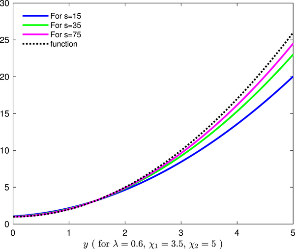
Let $g (y) = y^{2} + \frac{3}{4}$ , $ϰ_{1} = 3.5, ϰ_{2} = 5, λ = 0.6$ and $s \in {15, 35, 75}$ . Fig. 1 illustrates how the operator converges to the function $g (y)$ .

Example 5.2

Let $g (y) = (y - \frac{1}{3}) (y - \frac{3}{5})$ , $ϰ_{1} = 2, ϰ_{2} = 5, λ = 3$ and $s \in {15, 45, 75}$ . Fig. 2 illustrates how the operator converges towards $g (y)$ .

Convergence of the operator towards the function g ( y ) = y 2 + 3 4 .

These examples show us that when we take higher values of $s$ , the operators’ approximations of the function get better. Observe that the operators (2.2) reduce to operators (1.2) for $ϰ_{1} = ϰ_{2} = 0$ .

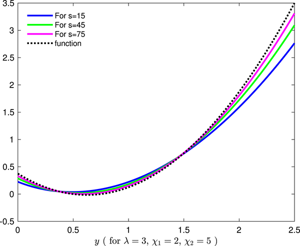
Convergence of the operator towards g ( y ) = ( y − 1 3 ) ( y − 3 5 ) .

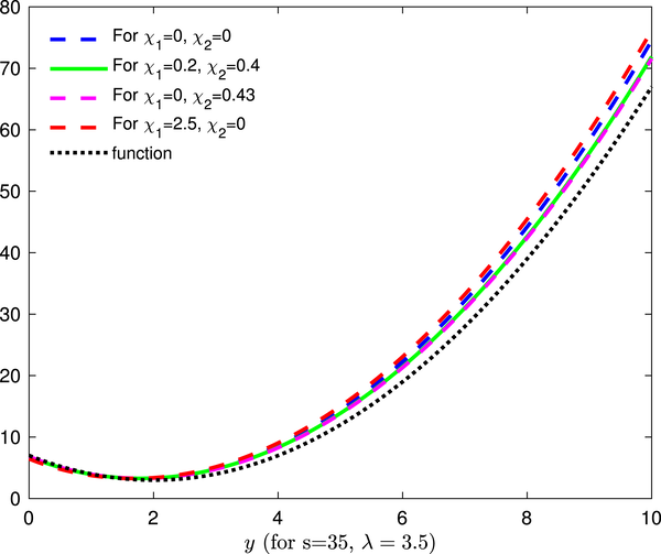
Comparison of convergence of the operator with the previous operator.

Example 5.3

Let $g (y) = y^{2} - 5 y + 9$ . For $λ = 3.5, s = 35$ comparison of convergence of constructed operator (1.6) Fig. 3 displays (green and pink) with the previously defined operator (1.5)(blue). This image clearly shows that the created operator provides a more accurate approximation to $g (y)$ than the operator that was previously specified.

6 Conclusion & observation

Our new operators (2.2) are the ones that we conclude in this article as the $λ$ -Bernstein Stancu type generated operators associated by shifted knots of Bézier basis function. For the selection of $ξ_{1} = ξ_{2} = 0$ in the equality (2.2), it is evident that our new operators $S_{s, λ}^{ϰ_{1}, ϰ_{2}}$ decreased to the most recent operators by the equality (1.4) (see Ayman-Mursaleen et al. (2024)). Additionally, for the choice of $ξ_{1} = ξ_{2} = 0$ and $ϰ_{1} = ϰ_{2} = 0$ the equality (2.2) reduced to the cited article (Cai et al., 2018) by equality (1.2) given by Cai et al. Based on these findings, we conclude that rather than (Ayman-Mursaleen et al., 2024; Bernstein, 2012; Cai et al., 2018 ), our novel operators are more generalized previous sorts of published research articles.

Funding

This research article did not receive any funding.

CRediT authorship contribution statement

Ahmed Alamer: Visualization, Funding acquisition. Md. Nasiruzzaman: Writing – review & editing, Writing – original draft.

Declaration of Generative AI and AI-assisted technologies in the writing process

The authors affirm that they did not utilize any artificial intelligence (AI) tools in the writing of this article.

Acknowledgments

Authors are extremely grateful to the reviewers for their valuable comments and crucial role in leading to a better presentation of this manuscript.

Declaration of competing interest

The authors declare that they have no known competing financial interests or personal relationships that could have appeared to influence the work reported in this paper.

References

Altomare F., . Korovkin type theorems and approximation by positive linear operators. Surv. Approx. Theory. 2010;5:92-164. DOI: Source
[Google Scholar]
Aslan R., Mursaleen M., . Some approximation results on a class of new type $λ$ -Bernstein polynomials. J. Math. Inequal.. 2022;16(2):445-462.
[Google Scholar]
Ayman-Mursaleen M., Kiliçman A., Nasiruzzaman M., . Approximation by $q$ -Bernstein-Stancu-Kantorovich operators with shifted knots of real parameters. Filomat. 2022;36:1179-1194.
[Google Scholar]
Ayman-Mursaleen M., Nasiruzzaman M., Rao N., Dilshad M., Nisar K.S., . Approximation by the modified $λ$ -Bernstein-polynomial in terms of basis function. AIMS Math.. 2024;9(2):4409--4426.
[Google Scholar]
Ayman-Mursaleen M., Rao N., Rani M., Kiliçman A., Al-Abied A.A.H.A., Malik P., . A note on approximation of blending type Bernstein– Schurer–Kantorovich operators with shape parameter $α$ . J. Math.. 2023;2023:5245806
[Google Scholar]
Barbosu D., . The Voronovskaja theorem for Bernstein-Schurer operators. Bull. Ştiinţ. Univ. Baia Mare Ser. B. 2002;18(2):137-140.
[Google Scholar]
Bernstein S.N., . Démonstration du théoréme de Weierstrass fondée sur le calcul des probabilités. Commun. Soc. Math. Kharkow.. 2012;2(13):1-2.
[Google Scholar]
Braha N., Mansour T., Mursaleen M., Acar T., . Convergence of $λ$ -Bernstein operators via power series summability method. J. Appl. Math. Comput.. 2020;65:125-146.
[Google Scholar]
Cai Q.B., Lian B.Y., Zhou G., . Approximation properties of $λ$ -Bernstein operators. J. Inequal. Appl.. 2018;2018:61.
[Google Scholar]
DeVore R.A., Lorentz G.G., . Constructive Approximation. Berlin: Springer; 1993.
Ditzian Z., Totik V., . Moduli of Smoothness. New York: Springer; 1987.
Gadjiev A.D., . The convergence problem for a sequence of positive linear operators on bounded sets and theorems analogous to that of P. P. Korovkin. Dokl. Akad. Nauk SSSRTransl. Sov. Math. Dokl.. 19741974;15:218.:1433-1436.
[Google Scholar]
Gadjiev A.D., Ghorbanalizadeh A.M., . Approximation properties of a new type Bernstein-Stancu polynomials of one and two variables. Appl. Math. Comput.. 2010;216:890-901.
[Google Scholar]
Gadziev A.D., . Theorems of the type of P.P. Korovkin’s theorems. Mat. ZametkiMath. Notes.. 19761976;20Mat. ZametkiMath. Notes.. 19761976;20:781-786.:995-998-786. (in Russian) (Engl. Trans.)
[Google Scholar]
Heshamuddin M., Kumar A., Rao N., Shadab M., Srivastava A., . Bivariate extension of $λ$ -Hybrid type operators. Ital. J. Pure Appl. Math.. 2023;49:271-292.
[Google Scholar]
Heshamuddin M., Rao N., Lamichhane B.P., Kilicman A., Ayman-Mursaleen M., . On one- and two-dimensional $α$ -Stancu-Schurer-Kantorovich operators and their approximation properties. Mathematics. 2022;10(8):3227.
[Google Scholar]
Korovkin P.P., . Convergence of linear positive operators in the spaces of continuous functions (Russian) Dokl. Akad. Nauk. SSSR (N.S.). 1953;90:961-964.
[Google Scholar]
Lenze B., . On Lipschitz type maximal functions and their smoothness spaces. Nederl. Akad. Indag. Math.. 1988;50:53--63.
[Google Scholar]
Mohiuddine S.A., Acar T., Alghamdi M.A., . Genuine modified Bernstein-Durrmeyer operators. J. Inequal. Appl.. 2018;2018:104.
[Google Scholar]
Mohiuddine S.A., Acar T., Alotaibi A., . Construction of a new family of Bernstein-Kantorovich operators. Math. Methods Appl. Sci.. 2017;40:7749-7759.
[Google Scholar]
Mohiuddine S.A., Özger F., . Approximation of functions by Stancu variant of Bernstein-Kantorovich operators based on shape parameter. Rev. R. Acad. Cienc. Exact. Fís. Nat. Ser. A. 2020;114:70.
[Google Scholar]
Ozarslan M.A., Aktuğlu H., . Local approximation for certain King type operators. Filomat. 2013;27:173-181.
[Google Scholar]
Özger F., . On new Bézier bases with Schurer polynomials and corresponding results in approximation theory. Commun. Fac. Sci. Univ. Ank. Ser. A1 Math. Stat.. 2020;69(1):376-393.
[Google Scholar]
Özger F., Srivastava H.M., Mohiuddine S.A., . Approximation of functions by a new class of generalized Bernstein–Schurer operators. Rev. R. Acad. Cienc. Exactas Fís. Nat., Ser. A. 2020;114:173.
[Google Scholar]
Rahman S., Mursaleen M., Acu A.M., . Approximation properties of $λ$ -Bernstein-Kantorovich operators with shifted knots. Math. Methods Appl. Sci.. 2019;42(11):4042-4053.
[Google Scholar]
Srivastava A., Bisht S., . Error estimates using higher modulus of smoothness in l p spaces. In: Mathematical, Computational Intelligence and Engineering Approaches for Tourism, Agriculture and Healthcare. Singapore: Springer; 2022. p. :147-158.
[Google Scholar]
Srivastava H.M., Özger F., Mohiuddine S.A., . Construction of Stancu-type Bernstein operators based on Bézier bases with shape parameter $λ$ . Symmetry. 2019;11(3):316.
[Google Scholar]
Ye, Z., Long, X., Zeng, X.M., 2010. Adjustment algorithms for Bézier curve and surface. In: International Conference on Computer Science and Education. Vol. 2010, pp. 1712–1716.
Zeng X.M., Cheng F., . On the rates of approximation of Bernstein type operators. J. Approx. Theory. 2001;109(2):242-256.
[Google Scholar]

Data availability

Introduction and preliminaries

Operators using Bézier bases and calculating fundamental moments

Convergence properties of operators S s , λ ϰ 1 , ϰ 2

Voronovskaja type asymptotic formula

Graphical analysis

Conclusion & observation

Funding

CRediT authorship contribution statement

Declaration of Generative AI and AI-assisted technologies in the writing process

Fulltext Views
6

PDF downloads
3

View/Download PDF
Download Citations

BibTeX
RIS

Show Sections

[1] Altomare F., . Korovkin type theorems and approximation by positive linear operators. Surv. Approx. Theory. 2010;5:92-164. DOI: Source
[Google Scholar]

[2] Aslan R., Mursaleen M., . Some approximation results on a class of new type $λ$ -Bernstein polynomials. J. Math. Inequal.. 2022;16(2):445-462.
[Google Scholar]

[3] Ayman-Mursaleen M., Kiliçman A., Nasiruzzaman M., . Approximation by $q$ -Bernstein-Stancu-Kantorovich operators with shifted knots of real parameters. Filomat. 2022;36:1179-1194.
[Google Scholar]

[4] Ayman-Mursaleen M., Nasiruzzaman M., Rao N., Dilshad M., Nisar K.S., . Approximation by the modified $λ$ -Bernstein-polynomial in terms of basis function. AIMS Math.. 2024;9(2):4409--4426.
[Google Scholar]

[5] Ayman-Mursaleen M., Rao N., Rani M., Kiliçman A., Al-Abied A.A.H.A., Malik P., . A note on approximation of blending type Bernstein– Schurer–Kantorovich operators with shape parameter $α$ . J. Math.. 2023;2023:5245806
[Google Scholar]

[6] Barbosu D., . The Voronovskaja theorem for Bernstein-Schurer operators. Bull. Ştiinţ. Univ. Baia Mare Ser. B. 2002;18(2):137-140.
[Google Scholar]

[7] Bernstein S.N., . Démonstration du théoréme de Weierstrass fondée sur le calcul des probabilités. Commun. Soc. Math. Kharkow.. 2012;2(13):1-2.
[Google Scholar]

[8] Braha N., Mansour T., Mursaleen M., Acar T., . Convergence of $λ$ -Bernstein operators via power series summability method. J. Appl. Math. Comput.. 2020;65:125-146.
[Google Scholar]

[9] Cai Q.B., Lian B.Y., Zhou G., . Approximation properties of $λ$ -Bernstein operators. J. Inequal. Appl.. 2018;2018:61.
[Google Scholar]

[10] DeVore R.A., Lorentz G.G., . Constructive Approximation. Berlin: Springer; 1993.

[11] Ditzian Z., Totik V., . Moduli of Smoothness. New York: Springer; 1987.

[12] Gadjiev A.D., . The convergence problem for a sequence of positive linear operators on bounded sets and theorems analogous to that of P. P. Korovkin. Dokl. Akad. Nauk SSSRTransl. Sov. Math. Dokl.. 19741974;15:218.:1433-1436.
[Google Scholar]

[13] Gadjiev A.D., Ghorbanalizadeh A.M., . Approximation properties of a new type Bernstein-Stancu polynomials of one and two variables. Appl. Math. Comput.. 2010;216:890-901.
[Google Scholar]

[14] Gadziev A.D., . Theorems of the type of P.P. Korovkin’s theorems. Mat. ZametkiMath. Notes.. 19761976;20Mat. ZametkiMath. Notes.. 19761976;20:781-786.:995-998-786. (in Russian) (Engl. Trans.)
[Google Scholar]

[15] Heshamuddin M., Kumar A., Rao N., Shadab M., Srivastava A., . Bivariate extension of $λ$ -Hybrid type operators. Ital. J. Pure Appl. Math.. 2023;49:271-292.
[Google Scholar]

[16] Heshamuddin M., Rao N., Lamichhane B.P., Kilicman A., Ayman-Mursaleen M., . On one- and two-dimensional $α$ -Stancu-Schurer-Kantorovich operators and their approximation properties. Mathematics. 2022;10(8):3227.
[Google Scholar]

[17] Korovkin P.P., . Convergence of linear positive operators in the spaces of continuous functions (Russian) Dokl. Akad. Nauk. SSSR (N.S.). 1953;90:961-964.
[Google Scholar]

[18] Lenze B., . On Lipschitz type maximal functions and their smoothness spaces. Nederl. Akad. Indag. Math.. 1988;50:53--63.
[Google Scholar]

[19] Mohiuddine S.A., Acar T., Alghamdi M.A., . Genuine modified Bernstein-Durrmeyer operators. J. Inequal. Appl.. 2018;2018:104.
[Google Scholar]

[20] Mohiuddine S.A., Acar T., Alotaibi A., . Construction of a new family of Bernstein-Kantorovich operators. Math. Methods Appl. Sci.. 2017;40:7749-7759.
[Google Scholar]

[21] Mohiuddine S.A., Özger F., . Approximation of functions by Stancu variant of Bernstein-Kantorovich operators based on shape parameter. Rev. R. Acad. Cienc. Exact. Fís. Nat. Ser. A. 2020;114:70.
[Google Scholar]

[22] Ozarslan M.A., Aktuğlu H., . Local approximation for certain King type operators. Filomat. 2013;27:173-181.
[Google Scholar]

[23] Özger F., . On new Bézier bases with Schurer polynomials and corresponding results in approximation theory. Commun. Fac. Sci. Univ. Ank. Ser. A1 Math. Stat.. 2020;69(1):376-393.
[Google Scholar]

[24] Özger F., Srivastava H.M., Mohiuddine S.A., . Approximation of functions by a new class of generalized Bernstein–Schurer operators. Rev. R. Acad. Cienc. Exactas Fís. Nat., Ser. A. 2020;114:173.
[Google Scholar]

[25] Rahman S., Mursaleen M., Acu A.M., . Approximation properties of $λ$ -Bernstein-Kantorovich operators with shifted knots. Math. Methods Appl. Sci.. 2019;42(11):4042-4053.
[Google Scholar]

[26] Srivastava A., Bisht S., . Error estimates using higher modulus of smoothness in l p spaces. In: Mathematical, Computational Intelligence and Engineering Approaches for Tourism, Agriculture and Healthcare. Singapore: Springer; 2022. p. :147-158.
[Google Scholar]

[27] Srivastava H.M., Özger F., Mohiuddine S.A., . Construction of Stancu-type Bernstein operators based on Bézier bases with shape parameter $λ$ . Symmetry. 2019;11(3):316.
[Google Scholar]

[28] Ye, Z., Long, X., Zeng, X.M., 2010. Adjustment algorithms for Bézier curve and surface. In: International Conference on Computer Science and Education. Vol. 2010, pp. 1712–1716.

[29] Zeng X.M., Cheng F., . On the rates of approximation of Bernstein type operators. J. Approx. Theory. 2001;109(2):242-256.
[Google Scholar]

Approximation by Stancu variant of λ -Bernstein shifted knots operators associated by Bézier basis function

Abstract

Keywords

41A25

41A36

33C45

Bernstein basis polynomial

Bézier basis function

λ-Bernstein-polynomial

Shifted knots

Stancu operators

Ditzian–Totik uniform modulus of smoothness

Lipschitz maximal functions

Peetre’s K-functional

Data availability

1 Introduction and preliminaries

2 Operators using Bézier bases and calculating fundamental moments

3 Convergence properties of operators S s , λ ϰ 1 , ϰ 2

Theorem 3.1 Altomare, 2010; Korovkin, 1953

Theorem 3.3 Gadziev, 1976; Gadjiev, 1974

Remark 3.5 DeVore and Lorentz, 1993

4 Voronovskaja type asymptotic formula

5 Graphical analysis

6 Conclusion & observation

Funding

CRediT authorship contribution statement

Declaration of Generative AI and AI-assisted technologies in the writing process

Acknowledgments

Declaration of competing interest

References

Suggested read for related articles:

Approximation by Stancu variant of $λ$ -Bernstein shifted knots operators associated by Bézier basis function

3 Convergence properties of operators $S_{s, λ}^{ϰ_{1}, ϰ_{2}}$