

Translate this page into:
Approximate analytical solutions for some obstacle problems
⁎Corresponding author at: Mathematics Department, College of Science and Arts, AlKamel, University of Jeddah, Saudi Arabia. chamekhmourad1@gmail.com (Mourad Chamekh),
-
Received: ,
Accepted: ,
This article was originally published by Elsevier and was migrated to Scientific Scholar after the change of Publisher.
Peer review under responsibility of King Saud University.
Abstract
The paper deals with the variational iteration method to obtain a semi-analytical solution to some obstacle problems. We will focus on applications of a contact problem for a deformed beam with an elastic obstacle. To validate the accuracy this approach,the obtained solution has been compared with the exact solution, in the case where it can be calculated in the closed-form expression. Otherwise, a comparison of variational iteration method with the Adomian decomposition method for some nonlinear examples has been used.
Keywords
Obstacle problems
Penalty function method
Variational Iteration Method
74K10
74M15
74S05

1 Introduction
Obstacle problems are problems well studied in many scientific literatures, including the problems of deformation of an elastic rod in the presence of an elastic or rigid obstacle (Caffarelli, 1998; Caffarelli and Figalli, 2013; Figalli and Serra, 2019). The resolution of the problems is either difficult, or too long to implement like the numerical problems of the contact in an elastic rod with or without friction (Chamekh et al., 2014; Chamekh, 2015; Chamekh et al., 2020a). Thanks to the penalization method, the obstacle problems are transformed into types of differential equations which can be solved by the Adomian decomposition method or the Variational Iteration Method (VIM), see Alderremy et al. (2019), Chamekh et al. (2020b) and Elzaki and Chamekh (2018).
This work emphasizes studies semi-analytical solutions related to obstacle problem. The term of obstacle problem is usually used for a classic motivating example in the analytical study of differential inequalities and free boundary problems. In the scientific literature, we can find a good number of applications that have a model that is built on the obstacle problem, such as the finances, the engineering problems, Stefan problem etc. For this purpose, for example, we can consult the following references Baxter and Rennie (1996), Brezzi et al. (1978) and Gupta (2003).
In this paper, the original idea had been to find a semi-analytical solution of the deformation of a beam in the presence of an elastic foundation. They answered that surround this engineering application must not prevent to apply these results to other specialties but, on the contrary, must pave the way for more complex obstacle problems. On the alternatives of Lagrange multiplier method, J. H. He has developed the variational iteration method (He, 1999) since the end of the last century. In scientific literature, the VIM is increasingly being used in different research types. For example, we mention the viscoelastic beams (Martin, 2016), behavior fluids (Chamekh and Elzaki, 2018) etc…
Amongst the engineering problems leading to an obstacle problem which were classically raised, the bending analysis of clamped–clamped Euler–Bernoulli beams, onto an elastic foundation and subject to an applied load. The goal is to find the deflexion, the maximum deflexion of this beam. This could also be in the case of a membrane but with an alternative form occupies a bounded domain of the plane with a rigid obstacle. Vertical displacement of the membrane is represented by the graph of a function of in . We then look for the equilibrium position taking the membrane subjected to an external force, under the non-penetration constraint on .
In the equilibrium state, if the membrane is out of contact with the obstacle, the elasticity produces a balance of the membrane tension and the surface of the membrane is described by U. If the membrane comes in contact with the obstacle, the function fulfills the curvatures of U. More generally, in monodimensional case, these discussed problems can induce the type of system
The obstacle problem has many extensions well-respected in the literature, particularly in the nonlinearity of the elastic reactions and/or the noncommutative effects are considered of the membrane, because of that, we have obtained the last possible generalized form. The function is continuous on and is the obstacle function. The system (1–2) results of the mathematical modeling of problems containing the contact, unilateral, obstacle, deformation, and/or free boundary value. In the remainder, some possibilities are discussed concerning the semi-analytical solutions of this type of system using the VIM.
2 Main equations
The penalty method is the most commonly used method of constraint handling. The goal is to take advantage of the fact that this penalty can reduce differential inequalities in the form of equalities. In this regard, by using the penalty technique which has been applied by Lewy-Stampacchia (Lewy and Stampacchia, 1969) to give the regularity of the solutions of the variational inequalities, the system (1) results in the equation given by:
In the following, for the sake of simplicity, we assume that the obstacle function
is known as follows (see Al-Said et al., 1996):
Upon substitution of (4) into (3) with taking into account the penalty function we finally obtain
3 Variational Iteration Method (VIM)
The VIM or the He’s method is a simple and however capable method for solving a wide class of nonlinear problems. It successfully has been applied to many problems. For example, He has utilized his method to solve the classical Blasius equation, a few well-known nonlinear problems, and ordinary differential systems. Presently, the VIM has been used in many fields, it is capable of handling a large class of linear or nonlinear differential equations. Adaptability and adjustment given by this method have made it promptly appropriate for cases where the analytical solutions are not available as is often the case in the applied sciences and engineering. The VIM gives effective calculation for analytic approximate solutions and numeric simulations for real-world applications in sciences. This method does not require the utilization of additive computation algorithms regularly utilized to confront the nonlinear terms as the Adomian decomposition method, which would complicate the analytical calculations. The VIM approaches directly the linear and nonlinear problems straightforwardly in the same way.
From He (1999), we recall the basic concept of VIM associated with the problem (5) follows the following iterative formula
4 Numerical examples
The proposed examples of the solutions of the linear and nonlinear problems show the effectiveness of the studied approach. The classical examples where we can give a closed-form solution that is possible enables us to evaluate the precision of calculated solutions.
4.1 Third-order linear obstacle problem
In the areas of oceanography (Al-Said et al., 1996), for example, the modeling can contribute to third-order differential equations. Taking
and
, with boundary conditions
, we obtain the following problem
From the variational formulation we can easily verify the regularity of solution in Sobolev space
of the next problem which is equivalent to problem (8) (see Al-Said et al., 1996):
The exact solution is as follows
We can now find the approximate solution of the problem (8) by using VIM. According to the iterative formula (6), we can write the problem (8) in the iterative form
Using the boundary conditions at 0, we obtain a possible parametric expression of
that is given by
Fig. 1 shows that the curve of the exact solution merges with that of the VIM solution. This precise result can be clearer in Fig. 2 where we notice that the order of the relative error is
. After the second iteration of VIM, we obtained satisfactory results, which indicates the effectiveness and high accuracy of this method for an optimal computing cost.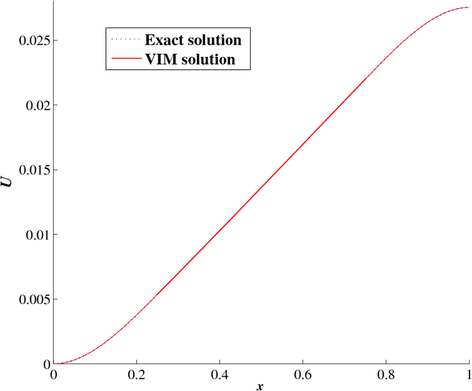
Comparing the exact solution in blue dashed-line with the two-iteration VIM solution in red straight-line.
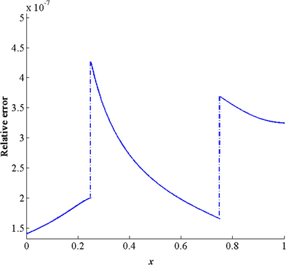
The curve of relative error.
4.2 Third-order nonlinear obstacle problem
In the next, we Take
and
, with boundary conditions
, under (5) we obtain the following problem
Fig. 3 shows that the curve of the Adomian solution merges with that of the VIM solution. It should be noted, however, that we have used the Adomian method for comparison purposes. This allows us to draw the following conclusion: The VIM and Adomian method give almost the same precision for this nonlinear problem of the obstacle.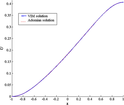
Comparing the two-iteration VIM solution in straight-line (blue), with the Adomian solution in dashed-line (red).
5 Conclusion
The differential inequalities which describe the obstacle problem are transformed into the differential equations thanks to the penalization method. The equations thus obtained were processed by the variational iteration method. The discussed examples of a beam with an elastic obstacle show some the major benefits: It leaves freedom of choice, on various loads, to an arbitrary point or region on the beam, on the boundary conditions at the ends of the beam; and the VIM is inexpensive and simple to implement and therefore the required programming skills are not necessary. We conclude the effectiveness and reliability of this method for solving certain type of these problems.
Acknowledgements
This work was funded by the University of Jeddah, Saudi Arabia, under Grant No. (UJ-20-DR-100). The authors, therefore, acknowledge with thanks the University technical and financial support changes.
Declaration of Competing Interest
The authors declare that they have no known competing financial interests or personal relationships that could have appeared to influence the work reported in this paper.
References
- Modified Adomian Decomposition Method to Solve Generalized Emden- Fowler Systems for Singular IVP. Math. Probl. Eng. 2019:6.
- [Google Scholar]
- Finite difference scheme for variational inequalities. J. Optim. Theory Appl.. 1996;89(2):453-459.
- [Google Scholar]
- Financial Calculus: An Introduction to Derivative Pricing. Cambridge, UK: Cambridge University Press; 1996.
- Error estimates for the finite element solution of variational inequalities. Part II. Mixed methods. Numer. Math.. 1978;31:1-16.
- [Google Scholar]
- Caffarelli, Luis, Figalli, Alessio, 2013. Regularity of solutions to the parabolic fractional obstacle problem. Journal für die reine und angewandte Mathematik (Crelles Journal). Volume 2013, Issue 680, Pages 191–233, ISSN (Online) 1435–5345, ISSN (Print) 0075–4102.
- Non-linear stability criterion in numerical approximation of hyperelastic rods Universal. J. Eng. Mech.. 2015;3:45-52.
- [Google Scholar]
- Explicit solution for some generalized fuids in laminar fow with slip boundary conditions. J. Math. Comput. Sci.. 2018;18:272-281.
- [Google Scholar]
- Stability of elastic rods with self-contact. Comput. Methods Appl. Mech. Eng.. 2014;279:227-246.
- [Google Scholar]
- Chamekh, M., Latrach, M.A. Renard, Y., 2020. Frictional self-contact problem of elastic rods. Journal of King Saud University-Science. Elsevier BV. 32, 828–835.
- Chamekh, M., Elzaki, T.M., Brik, N., 2020. Semi–analytical solution for some proportional delay diferential equations, SN Appl. Sci., 148 (2019), 6 pages 1.
- Solving nonlinear fractional differential equations using a new decomposition method. Univ. J. Appl. Math. Comput.. 2018;6:27-35.
- [Google Scholar]
- On the fine structure of the free boundary for the classical obstacle problem. Invent. Math.. 2019;215:311-366.
- [Google Scholar]
- The Classical Stefan Problem: Basic Concepts, Modelling and Analysis. Amsterdam: Elsevier; 2003.
- Variational iteration method a kind of nonlinear analytical technique: some examples. Int. J. Nonlinear Mech.. 1999;34:699-708.
- [Google Scholar]
- On the regularity of the solution of a variational inequality. Commun. Pure Appl. Math.. 1969;22(2):153-188.
- [Google Scholar]
- A modified variational iteration method for the analysis of viscoelastic beams. Appl. Math. Model.. 2016;40(17–18):7988-7995.
- [Google Scholar]


