

Translate this page into:
Applications of new integral transform for linear and nonlinear fractional partial differential equations
⁎Corresponding author. Tarig.alzaki@gmail.com (Tarig M. Elzaki)
-
Received: ,
Accepted: ,
This article was originally published by Elsevier and was migrated to Scientific Scholar after the change of Publisher.
Peer review under responsibility of King Saud University.
Abstract
This study aims to obtain the approximate resolution of the fractional partial differential equation through the help of unprecedented new integral transform (NIT) called Elzaki Decomposition Method (EDM), applied to the new integral transform for fractional partial differential equations (PDEs). The technique converges to the right solution, fractional partial differential equations. Some examples were illustrated to confirm the accuracy of the method.
Keywords
Fractional partial differential equation
New integral transform method (NIT)
Adomian decomposition method (ADM)

1 Introduction
Many of phenomena emerging from many scientific displaces such as plasma physics, solid state physics, mathematical biology, fluid dynamics and chemical kinetic are technicality partial differential equation (Miller and Ross, 1993; Podlubny, 1999; Mahdy et al., 2015).
The new integral transform was proposed by tarig Elzaki to enable solving ordinary and partial differential equation in time domain. Several mathematical tools can be used to solve differential equation like Fourier, Laplace and Sumudu transform (Elzaki, 2011; Mohamed and Elzaki, 2014). For a broad spectrum of functional equations, (ADM) is used with success (Adomian, 1994). This method relies on infinite series to represent a solution and it is often the case where the series converges to the accurate solution. In (Bulut and Evans, 2002); (ADM) is applied to dissolve differential equation. (El-Tawil et al., 2004) solved the differential equation and then obtained results that were compared to the results obtained by using standard (ADM). In this dissertation, we applied (NIT) method to obtained accurate analytical and approximate solutions to equation of fractional order.
The paper is structured as follows: in Section 2, the foundations of the fractional calculus are presented. In Section 3, the methodology of the study, we used (NIT) algorithm for PDEs. Section 4 contains the efficiency and strength of the method with illustrative examples showing it. Stopping points are offered in Section 5.
2 Fundamental concepts of fractional theory
In this segment, we remark the subject requisite definitions and attributes of the fractional calculus theory and ELzaki Transform.
A function is told to be in the space if the yonder be a real number such that where clearly
let’s Riemann-Liouville fractional integral operator of order
then
is known as, accordingly (Miller and Ross, 1993; Podlubny, 1999; Mahdy et al., 2015);
Caputo fractional derivative of the left sided,
is known as, accordingly
we hold properties of the operator (Miller and Ross, 1993; Podlubny, 1999; Mahdy et al., 2015; Elzaki, 2011; Mohamed and Elzaki, 2014; Adomian, 1994; Bulut and Evans, 2002; El-Tawil et al., 2004; Arife and Yildirim, 2011; He, 1997; He, 1997; He, 1998; He, 1998; He, 1999; Wazwaz, 2007);
the new integral transform (NIT) is known as, accordingly (Elzaki, 2011; Mohamed and Elzaki, 2014);
Before the next formulation,
If
then the new integral transform (NIT) of the fractional derivative
is,
where be the (NIT) (Mohamed and Elzaki, 2014).
3 The new integral decomposition (NIT)
The purpose of this subdivision is to talk about the use of The (NIT) algorithm for linear and nonlinear fractional partial differential equation. We take the universal form of inhomogeneous linear and Non-linear Partial Fractional differential equations of the frame.
Applying the (NIT) to both parties of Eq. (3.1), and referring to the linearity of the (NIT), the result is:
Applying the (NIT) property, we will get:
Suppose
to will get
The criterion of the new integral decomposition method defines the solution
in sequences
The Non-linear Formula is Decomposition as, accordingly:
For the nonlinear, function
the first Adomian polynomials (Adomian, 1994), to will get:
Finally, by using the two parties of the equation, we get the repeated algorithm as the following
As accordingly, we conclude that the repeating relation is specified by:
Applying the inverse (NIT) Eqs. (3.8)–(3.11), to obtain:
In which is the function that comes from the origin term and the specific initial condition. Now first applying The (NIT) of the terms on the right hand side of Eq. (3.13) then applying inverse Elzaki transform we get the value of .
4 Illustrative examples
In this segment, we use the fractional new integral transform decomposition method for solving Time- Fractional PDEs in a pipe.
Consider the following one-dimensional linear inhomogeneous fractional wave equation (Adomian, 1994).
Subject to the initial condition:
Applying the (NIT) to both parties Eq. (4.1), to get:
Using given initial condition Eq. (4.3), become
For the nonlinear, function
the first Adomian polynomials (Adomian, 1994), to obtain:
Finally, by using the two parties of the Eq. (4.5), we get the repeated algorithm as the following
Applying the inverse (NIT) Eqs. (4.6) and (4.7), to obtain:
Consequently,
By excluding the noise terms and holding the part that contains the non-noise terms, we get the accurate solution of the Eq. (4.1). Starting by , and repeating the process twice, we obtain the accurate solution .
Consider the following one-dimensional linear inhomogeneous fractional Burgers equation (Odibat and Momani, 2009);
Subject to the initial condition:
Applying the (NIT) to both parties Eq. (4.12), to get:
Using given initial condition Eq. (5.14) become,
The nonlinear function
the first Adomian polynomials (Adomian, 1994), to obtain;
Finally, by using the two parties of the Eq. (4.16), we get the repeated algorithm as the following:
Applying the inverse (NIT) Eqs. (4.17) and (4.18), to obtain:
Consequently,
Canceled noise terms of satisfy Eq. (4.12), we find that the exact solution is given by
Consider the following nonlinear Time- Fraction KdV equation (Wazwaz, 2007)
Subject to the initial condition:
Applying the (NIT) to both parties Eq. (4.23), we will get:
Using the given initial condition, Eq. (4.25) become,
The first few components of polynomials are given by:
Finally, by using the two parties of the Eq. (4.27), we get the repeated algorithm as the following:
Applying the inverse (NIT) for Eqs. (4.28) and (4.29), to obtain:
Consequently,
The other components of the EDM competence are determined in an identical format, then approximate solution of (4.23) in sequence,
And when we obtain the exact solution of the nonlinear KdV Equation (Wazwaz, 2007) (see Table 1 and Fig. 1).
Consider the following nonlinear Time- Fraction differential equation (Wazwaz, 2007);
Subject to initial condition:
Applying the (NIT) to both parties Eq. (4.31), we will get:
Using given initial condition Eq. (4.33) become,
The Nonlinear function
the first Adomian polynomials (Adomian, 1994), to will get
The first few components of
polynomials are given by:
Finally, by using the two parties of the Eq. (4.35), we get the repeated algorithm as the following
Applying the inverse (NIT) Eqs. (4.37) and (4.38), to obtain:
Consequently,
When
Eq. (4.42) becomes:
On the side, we catch sight of that the development of the function
according to the Taylor series in the vicinity of
is will get:
Therefore, we conclude that: that is the accurate solution of Eq. (4.31) in the status (see Table 2 and Fig. 2).
| 0.01 | 0 0.1000 | 0 | 0 | 0 | 0 | 0 |
| 0.2000 | 1.0237 | 0.9935 | 0.9658 | 0.9404 | 0.9375 | |
| 0.3000 | 2.0474 | 1.9871 | 1.9317 | 1.8808 | 1.8750 | |
| 0.4000 | 3.0711 | 2.9806 | 2.8975 | 2.8212 | 2.8125 | |
| 0.5000 | 4.0949 | 3.9742 | 3.8634 | 3.7617 | 3.7500 | |
| 0.6000 | 5.1186 | 4.9677 | 4.8292 | 4.7021 | 4.6875 | |
| 0.7000 | 6.1423 | 5.9612 | 5.7951 | 5.6425 | 5.6250 | |
| 0.8000 | 7.1660 | 6.9548 | 6.7609 | 6.5829 | 6.5625 | |
| 0.9000 | 8.1897 | 7.9483 | 7.7268 | 7.5233 | 7.5000 | |
| 1.0000 | 9.2134 | 8.9419 | 8.6926 | 8.4637 | 8.4375 | |
| 10.2372 | 9.9354 | 9.6585 | 9.4042 | 9.3750 | ||
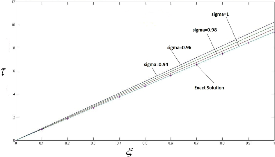
- The plot of solution of Example 4.3, when
and
.
| 1.1 | 0 | 0 | 0 | 0 | 0 | 0 |
| 0.1000 | 0.1105 | 0.1105 | 0.1105 | 0.1104 | 0.1104 | |
| 0.2000 | 0.2239 | 0.2238 | 0.2237 | 0.2236 | 0.2236 | |
| 0.3000 | 0.3435 | 0.3432 | 0.3429 | 0.3425 | 0.3425 | |
| 0.4000 | 0.4735 | 0.4726 | 0.4718 | 0.4709 | 0.4708 | |
| 0.5000 | 0.6197 | 0.6176 | 0.6156 | 0.6137 | 0.6131 | |
| 0.6000 | 0.7906 | 0.7862 | 0.7820 | 0.7781 | 0.7761 | |
| 0.7000 | 0.9993 | 0.9906 | 0.9824 | 0.9745 | 0.9697 | |
| 0.8000 | 1.2659 | 1.2493 | 1.2337 | 1.2190 | 1.2097 | |
| 0.9000 | 1.6208 | 1.5902 | 1.5616 | 1.5348 | 1.5237 | |
| 1.0000 | 2.1086 | 2.0540 | 2.0033 | 1.9560 | 1.9648 | |
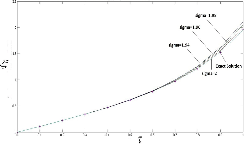
- The plot of solution of Example 4.4 when,
and
.
5 Conclusions
New transform decomposition method has been utilized to apply to find an exact solution of Fractional Partial Differential Equations, with constant coefficients. Definitions and theorems are introduced, and special formulas of Mittage -Leffler function are observed with their proofs, it is concluded that the new decomposition transform is a potent, effective and reliable instrument to determine the resolution of fractional partial differential equations.
References
- Solving Frontier Problems of Physics: The Decomposition Method. Dordrecht: Kluwer Academic Publishers; 1994.
- New modified variational iteration transform method (MVITM) for solving eighth-order boundary value problems in one step. World Appl. Sci. J.. 2011;13(10):2186-2190.
- [Google Scholar]
- On the solution of the Riccati equation by the decomposition method. Int. J. Comput. Math.. 2002;79:103-109.
- [Google Scholar]
- The new integral transform “ELzaki Transform”. Global J. Pure Appl. Math.. 2011;7(1):57-64. ISSN 0973–1768
- [Google Scholar]
- Solving Riccati differential equation using Adomian’s decomposition method. Appl. Math. Comput.. 2004;157:503-514.
- [Google Scholar]
- Variational iteration method for delay differential equations. Commun. Nonlinear Sci. Numer. Simul.. 1997;2(4):235-236.
- [Google Scholar]
- Semi-inverse method of establishing generalized principles for fluid mechanics with emphasis on turbo machineryaero dynamics. Int. J. Turbo Jet-Engines. 1997;14(1):23-28.
- [Google Scholar]
- approximate solution of nonlinear differential equations with convolution product nonlinearities. Comput. Meth. Appl. Mech. Eng.. 1998;167:69-73.
- [Google Scholar]
- approximate analytical solution for seepage flow with fractional derivatives in porous media. Comput. Meth. Appl. Mech. Eng.. 1998;167:57-68.
- [Google Scholar]
- Variational iteration method – a kind of non-linear analytical technique: some examples. Int. J. Nonlinear Mech.. 1999;34:699-708.
- [Google Scholar]
- Implementation of the homotopy perturbation sumudu transform method for solving klein-gordon equation. Appl. Math.. 2015;6:617-628.
- [Google Scholar]
- An Introduction to the Fractional Calculus and Fractional Differential Equations. New York: John Wiley and Sons; 1993.
- Solutions of fractional ordinary differential equations by using Elzaki transform. Appl. Math.. 2014;9(1):27-33. ISSN 0973–4554
- [Google Scholar]
- The variational iteration method: An efficient scheme for handling fractional partial differential equations in fluid mechanics. Comput. Math. Appl.. 2009;58:2199-2208.
- [Google Scholar]
- Fractional Differential Equations. San Diego, CA: Academic Press; 1999.
- The variational iteration method for rational solutions for KdV, K(2,2), Burgers, and cubic Boussinesqequations. J. Comput. Appl. Math. 2007;207:18-23.
- [Google Scholar]


