

Translate this page into:
Application of interpolation finite element methods to a real 3D leaf data
-
Received: ,
Accepted: ,
This article was originally published by Elsevier and was migrated to Scientific Scholar after the change of Publisher.
Peer review under responsibility of King Saud University.
Abstract
In this paper we proposed a new surface fitting method based on combining the Clough-Tocher method (CT) and multiquadric radial basis function enhanced with a cubic polynomial (MRBFC) method to accurately reconstruct a real leaf surface from 3D scattered data. The accuracy of the CT-MRBFC method is validated by implementing it to a real 3D leaf data.
The accuracy of the method depends highly on the RBF shape parameter and the triangular mesh structure. Consequently we employed three different methods numerically to estimate the RBF parameter as variable or constant including the square root method, the cubic root method and the fminbnd method which is a MATLAB command based on minimizing a single-variable function locally on a fixed interval. Moreover, the quality of the triangles in the mesh is measured to ensure that each triangle is close to equilateral triangle to achieve a better accuracy of the proposed CT-MRBFC method. It is concluded that the proposed CT-RBFC method generates an accurate representation of the leaf surface.
Keywords
Interpolation
Finite elements methods
Radial basis function
Clough-Tocher method

1 Introduction
The aim of the present paper is the application of surface fitting methods to generate a leaf surface. Leaf models have been researched widely by Kempthorne et al. (2015a,b, 2015), Oqiela and Ogilat (2018). Recently, Oqielat et al. (2007), Oqielat et al. (2009), Oqielat (2017) presented a model for the surface of leaf using finite elements method based on hybrid Clough-Tocher radial basis function method. Moreover, Oqielat and Ogilat (2017), Oqielat, (2018) implemented Hardy’s multiquadrics RBF interpolant to model the leaf surface. Kempthorne et al. (2015a) applied discrete smoothing -splines to build the surface of wheat and cotton leaves. The leaf model can be used to simulate the water droplet path on the leaf surface (Oqielat et al., 2011; Dorr et al., 2014; Lisa et al., 2016).
Two interpolation methods for surface fitting have been investigated in this article including Clough-Tocher method (CT) and radial basis function (RBF) method. Afterward, we proposed a hybrid method (CT-MRBFC) that joins the CT method and multiquadric RBF enhanced with a cubic polynomial method. The proposed CT-MRBFC method is then applied to reconstruct the surface of real leaf from 3D scanned data. The CT method is finite element method based on surface triangulation and requires derivative computing at the vertices and midpoints of the triangular elements. Therefore the multiquadric RBF enhanced with a cubic polynomial is used to estimate the necessary derivative for the CT method.
The RBF shape parameter has great influence on the accuracy of the RBF so we compared three methods to estimate the RBF parameter. Furthermore, a triangulation of the surface is essential to apply the proposed method where we introduced a methodology for triangulation that assure each triangle in the mesh is equilateral to obtain a more accurate representation of the surface. Finally, the hybrid CT-MRBFC method is validated using a real 3D data points sampled from Anthurium leaf.
This paper consists of four main sections. In Section 1, outline of the CT method, multiquadric RBF enhanced with a cubic polynomial method and the RBF parameter as a constant or variable is given. In Section 2, the CT-MRBFC method is proposed locally and globally. Moreover, a numerical investigation to measure the accuracy of the method is presented. In Section 3, the application of the CT-MRBFC method on the Anthurium leaf data set is exhibited where a triangulation methodology for the leaf surface and a new reference plane for the leaf data points are also given in this section. The results and conclusion are presented in Section 4.
1.1 The Clough-Tocher method
The Clough-Tocher (CT) technique (Clough, 1965) is an interpolation finite element approach based on triangulation of the data on a given domain to develop elements on which interpolants can be build. The triangle in the CT method is divided into three sub triangles (see Fig. 1) where a cubic polynomial is constructed on each sub triangle to facilitate piecewise cubic to be formulated over the whole domain which is continuous and differentiable, see Oqielat et al. (2009), Oqielat et al. (2007). Finite element methods have been researched broadly by Tinh et al. (2014); Tinh et al. (2016), Minh et al. (2016), Minh et al. (2017a,b). More information about CT method can be found in Lancaster (1986), the interpolation CT is defined by
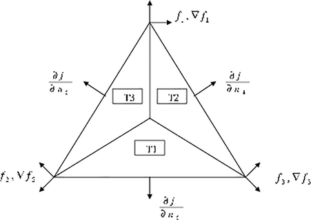
The clough-tocher triangle.
1.2 Radial basis function approximation with polynomial reproduction
The RBF approximation to
is a function
of the form
and
RBF method introduced by Hardy (1990), its offer a smooth surface by producing a good estimate of the function values at the surface points. The most common use RBF’s including thin plate splines, Gaussian RBF and Hardy’s multiquadric. In this paper we adopted the multiquadric RBF (Hardy, 1990) which is given by:
1.2.1 Constant and variable shape parameter
Many researchers studied the influence of the RBF parameter α on the RBF accuracy and found that it has a large impact on the quality of the RBF approximation where for some α the system given in Eq. (3) becomes ill-conditioned. Majdisova et al. (2017) suggested a RBF for large data sets where α was defined experimentally.
The variable shape parameter methodology allows the user to obtain a diverse value of the parameter at each centre of the RBF which conduct well-conditioned system, see Eq. (3). However, using a variable shape parameter sometimes leads to possibly singular and non-symmetric linear system whereas using a constant shape parameter produces invertible system. Sarra and Sturgill (2009), Golbabai and Rabeie (2012) suggested sinusoidal parameter given by
A polynomial
of degree (
) can be added to the RBF interpolant to improve the method accuracy, therefore in this research we added a polynomial of degree three to the multiquadric RBF given by:
2 Hybrid Clough-Tocher multiquadric radial basis function enhanced with a cubic polynomial method
In this paper, we introduced a new hybrid interpolation approach that combine the Clough-Tocher and multiquadric RBF enhanced with a cubic polynomial methods (CT-MRBFC) to achieve a smooth and accurate representation of the surface. This combination allow us to estimate the gradients requires for the CT-triangle using multiquadric RBF enhanced with a cubic polynomial as follows:
The gradient of the MRBFC
given in Eq. (8) is given by
The advantage of the CT-MRBFC method is that it results in a continuous and smooth surface representation as well as the method provides a decent precision adjacent the boundary of their domain.
2.1 Numerical experiment for the Franke data
In this section, the outcomes of our numerical investigation for the proposed CT-MRBFC is presented. The precision of the CT-MRBFC method is measured using a data taken from Franke (1982). The data consist of two sets of points and three test function. The first set includes 100 points defined on a unit square where this set is used to built a surface triangulation for the CT method (see Oqielat et al., 2007; Oqielat et al., 2009) while the second set comprises of 33 points. The CT-MRBFC method assessed using the 33 points by computing the error of the root mean square (RMSE) given by:
The local MRBFC method that uses point and the global MRBFC method that uses point are employed to approximate the gradients for the CT triangle. The shape parameter was computed either locally using variety of adjacent points to the center of the CT triangle or globally using points (see Tables 2 and 3).
In this paper we investigated three techniques to estimate the parameter ( ) locally and globally. These methods are the fminbnd method, the square root (SR) method (Eq. (7)) and the cubic root (SR) method (Eq. (6)). The fminbnd method is a MATLAB command based on minimizing a single-variable function locally on a fixed interval either by the trisection approach that divides the interval into three equal parts or by the bisection approach twice on the interval. The numerical experiments given in the following section shows that using fminbnd in the CT-MRBFC method produces more accurate RMS than using the CR and SR method.
Tables 2 and 3 show the results of applying the global and the local CT-MRBFC method via computing the RMS errors for the three test functions. The RBF shape parameter in Tables 2 and 3 estimated globally using (N = 100) points by Fminbnd, square root parameter (SR) and Cubic root parameter (CR) while in Table 4 the parameter was estimated locally using m = 40 points.
We observe from Table 2 that using the global CT-MRBFC method creates RMS error accurately same as the exact gradients shown in Table 1, while the RMS error almost as good as the exact gradients for the local CT-MRBFC approach. Moreover, the RMS errors produces using global CT-MRBFC is slightly better than the RMS error obtained by local CT-MRBFC knowing that the parameter
computed globally using Fminbnd in both methods.
Function
Exact Gradient
1.4e−4
4.1e−5
44.4e−5
The observations in Table 3 show that the RMS obtained using global CT-MRBFC method is more accurate than the RMS acquired by the local CT-MRBFC for both cases (either using SR or CR to estimate the parameter
). Moreover, in both global and local method, employing the SR method produced better RMS error than using CR method. In our numerical investigation the shape parameter obtained using the CR method was
and it was
using the SR method on an interval
.
Functions
C
Global CT-MRBFC
Local CT-MRBFC
F3
0.5012
1.4e−004
1.5e−004
F4
1.0377
4.1e−005
4.2e−005
F6
1.5422
4.4e−005
4.8e−005
Functions
Quadratic root shape parameter
Cubic root shape parameter
Global CT-MRBFC
Local CT-MRBFC
Global CT-MRBFC
Local CT-MRBFC
F3
5.0e−004
5.2e−004
7.8e−004
8.0e−004
F4
1.9e−004
9.0e−004
1.3e−004
1.3e−004
F6
2.2e−003
2.7e−003
2.9e−003
3.6e−003
Table 4 shows a comparison between the RMS error for the three test function by local CT-MRBFC method,
computed locally using m = 40 points using the Fminbnd method, SR method and CR method. One observes from Table 4 is that using the local CT-MRBFC method yielded the best RMS error obtained when
estimated by fminbnd method, followed by the SR method and then the CR method. Furthermore, the interval of the
values achieved using the local CT-MRBFC method is given in the table. As we expect, the
values computed globally (Table 2) were always occur in the local interval of
given for each of the functions. However, computing
globally is less computationally costly than computing
locally since a new
value must be computed each time the local MRBFC is build.
Function
Local CT-MRBFC method (m = 40)
Using Fminbnd method
Quadratic root method
Cubic root method
[c_minc_max]
RMS
[c_minc_max]
RMS
[c_minc_max]
RMS
F3
[0.46 1.4]
1.5e−004
[0.01 0.3]
7.2e−004
[0.006 0.1]
8.5e−004
F4
[0.85 1.4]
4.1e−005
[0.04 1.2]
1.6e−004
[0.026 0.7]
1.9e−004
F6
[1.13 1.6]
5.2e−005
[0.10 2.9]
5.1e−004
[0.065 1.9]
6.9e−004
In conclusion, the RMS error produced using the global CT-MRBFC method, computed globally using fminbnd, is more accurate than all other method tested. Now, we pass this results to the next section and we investigate the appropriateness of the global CT-MRBFC method on a real data collected from real leaf.
2.2 Local and global CT-MRBFC approximations
In this framework two types of CT-MRBFC method are investigated which we denote to as the local and the global CT-MRBFC. The global CT-MRBFC based on using (n) points to formulate a global interpolation multiquadric RBF enhanced with a cubic polynomial (global MRBFC)
, then
is used to estimate the gradients for the clough-Tocher triangles. Though, for the local CT-MRBFC, a local subsets of bulk m = 40 of the entire data points (say N) is implemented to create a local MRBFC
for each triangle. Subsequently, the
is used to compute the gradients for the CT element. In this paper, the (m) points are the closest points to the vertices and edge midpoints of the interest CT element. The steps of implementation the hybrid CT-MRBFC method is outlined in the following algorithm
Algorithm 1: The CT-MRBFC Method for leaf Surface reconstruction
INPUT:
data points
Step 1: chose a subset of
data points to triangulae the surface.
Step 2: measure the quality of the triangle in the mesh using formula (15) to ensure that each
triangle is close to equilateral.
Step 3: compuate the MRBF given in Eq. (3) Using either a global MRBF from
points or a
local MRBF construct on each triangle from
points.
Step 4: use the Pseudoinverse technique to solve the linear system.
Step 5: use the RBF coefficients to estimate the local or the global derivative of the CT interpolant
Step 6: employ the CT-MRBFC method either locally
Or globally
to construct the
leaf surface
3 Application of the CT-MRBFC technique to a real leaf data set
To reconstruct the surface of a leaf using interpolation methods, it requires a collection of points sampled from the leaf surface. Loch (2004) used a laser scanner to collect the surface points of the Anthurium leaf. The Anthurium leaf data comprises of two sets, the first set includes 4,688 surface points (Fig. 2) and 106 boundary points for the second set, see Fig. 3(a). The accuracy of the hybrid Clough-Tocher multiquadric RBF enhanced with a cubic polynomial method (CT-MRBFC) proposed in Section 2 is evaluated using the Anthurium leaf data. Two phases are essential to be able to apply the CT-MRBFC technique to the leaf data, which contains determination of a new reference plane for the leaf data and then triangulation for the surface of the leaf.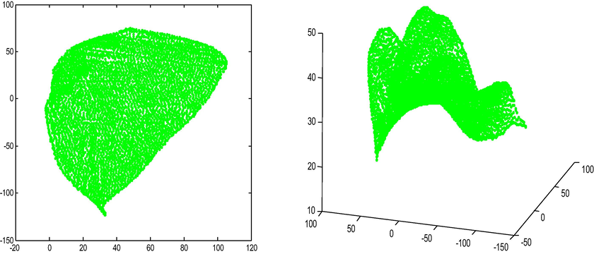
The 4,688 scanned Anthurium leaf points in 2D and 3D.
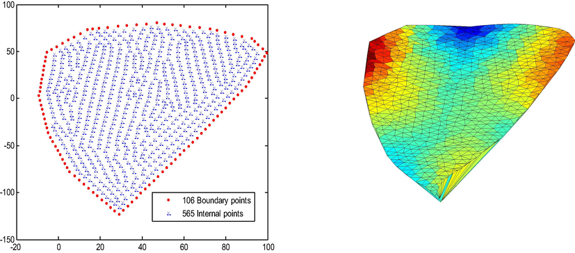
(a) Represent the 762 vertix point of the Anthurium leaf including 106 boundary points and 565 interior point. (b) The corresponding triangulation of the 762 points.
3.1 Leaf reference plane
The sampled leaf points reference plane does not coincide with the x,y-plane coordinate system, so to overcome this issue a reference plane that is the orthogonal distance regression plane fit to the sampled points is used (Oqiela and Ogilat, 2018).
Given data points
, fit
by the following orthogonal distance regression plane:
Find
that minimize
by evaluating the partial derivative with respect to
to be zero,
where
is the data points center which lies in the plane. Subsequently, Eq. (13) becomes
Eq. (14) can be represented in matrix form as follow:
Let then .
Finally, after we projected the data points into the new reference plane, we rotated the coordinate system using a rotation matrix (see Oqielat et al., 2009) to obtain the xy-plane as a new reference plane to the leaf data.
3.2 Triangulation of the leaf surface
The shape of the triangle in the mesh can be detrimental to the overall accuracy of the leaf surface fit. This problem is well known in the finite element literature (Clough, 1965; Lancaster, 1986). The CT-MRBFC method computational expenses can be decreased by choosing a subset of 762 points from the Anthurium data to triangulate the leaf surface. In the model presented here the mesh generation is curried out to ensure that every triangle is close to equilateral as possible. This should help to reduce the error since it reduces a multiplicative term in a theoretical error bound. So to get some indication of how good or bad is the RMSE and the representation of the leaf surface, it is useful to evaluate the quality of the mesh which is based on measuring the quality of each triangle in the mesh. One way to measure the quality (Daniel, 2005) of the element is:
In this context we perform a numerical experiment on one equilateral triangle to measure the quality of the mesh. We started with equilateral triangle and we finished with a thin triangle, see Fig. 4(a). The CT approximation value is evaluated at a point
close to the center of the equilateral triangle. Afterward, the height of the equilateral triangle
) is reduced toward its base (see Fig. 4(a)) and we compute the CT approximation value again at a point
close to the center of the new triangle. This process is repeated and each time we evaluate the CT approximation value, the exact value at that point is computed using the test function
, (where
to measure the error, the RMS error and the triangle quality, see Table 5. One observes from Table 5 that each time we reduced the height of the triangle, the quality of the triangle decreased and the error increased (see Fig. 4(b)). The final Triangulation of the Anthurium leaf is shown in Fig. 3(b).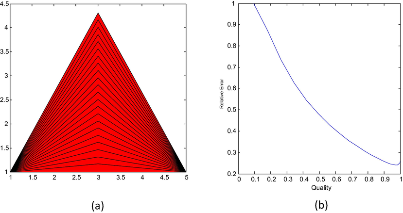
(a) Represent equilateral triangle where the height of the triangle reduced toward its base, (b) represent the relation of the triangle quality with the relative error of the CT method.
Exact value
CT value
RMS error
Triangle quality
−0.1391
−0.0831
0.2568
0.9990
−0.1334
−0.0812
0.2496
0.9959
−0.1276
−0.0787
0.2446
0.9904
−0.1217
−0.0757
0.2417
0.9822
−0.1158
−0.0721
0.2410
0.9710
−0.1098
−0.0681
0.2425
0.9564
−0.1037
−0.0637
0.2464
0.9382
−0.0976
−0.0590
0.2528
0.9159
−0.0915
−0.0540
0.2617
0.8893
−0.0854
−0.0488
0.2735
0.8581
−0.0793
−0.0435
0.2884
0.8220
−0.0732
−0.0380
0.3067
0.7806
−0.0671
−0.0325
0.3292
0.7340
−0.0611
−0.0270
0.3564
0.6818
−0.0551
−0.0215
0.3896
0.6243
−0.0492
−0.0160
0.4304
0.5614
−0.0434
−0.0107
0.4811
0.4934
−0.0377
−0.0055
0.5452
0.4207
−0.0321
−0.0006
0.6275
0.3437
−0.0266
0.0040
0.7349
0.2632
−0.0212
0.0078
0.8729
0.1799
−0.0160
0.0091
1.0000
0.0945
3.3 Numerical experiments for the leaf surface
The outcomes of employing the CT-MRBFC method to the data points sampled from Anthurium leaf is presented in this section. The accuracy of the CT-MRBFC method is evaluated using the remaining leaf points (say s) after selection the triangulation points by the RMS error given in Eq. (11) and the maximum error combined with the surface fit given in the following equation
Table 6 represent the maximum error and the RMS error by the CT-MRBFC method for the data points sampled from the Anthurium leaf. Note that the triangular mesh consists of 1486 triangles, given a total of 3793 point to measure the approximation of the proposed method. Furthermore, the maximum error obtained by the CT-MRBFC technique is less accurate than the RMS error. The optimal value of the multiquadric RBF is computed using Fminbnd and it was 2.9953. In conclusion, the CT-MRBFC method produces an accurate depiction of the Anthurium leaf (see Fig. 5)
Global CT-MRBF With Cubic Polynomial (Anthurium leaf)
Maximum error
4.4e−002
Relative RMS
8.9e−003
Number of point tested
3688
Number of Boundary points
106
The RBF Parameter (α)
2.9953
Triangulation points
762
Number of triangles
1486
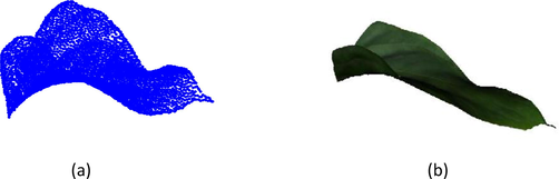
(a) The leaf surface model of the Anthurium leaf created using the Global CT-MRBF With Cubic Polynomial method. (b) The corresponding visualization of the leaf.
4 Results and conclusions
A new surface fitting method (CT-MRBFC) based on combining the Clough-Tocher method (CT) and multiquadric RBF method enhanced with a cubic polynomial (MRBFC) to model the leaf surface is presented. The CT-MRBFC method is applied to reconstruct the Anthurium leaf surface from 3D scanned points and it’s provide an accurate leaf representation, see Fig. 5. The leaf model can be used later to model a droplet of fluid (water or pesticide) movements on a leaf surface.
Acknowledgment
The author wish to thank the reviewer for the perceptive comments on the manuscript that developed the final appearance of the paper.
References
- Belward, J. Turner, I. Oqielat, M., 2008. Numerical investigation of linear least square methods for derivatives estimation. In: CTAC 08 Computational Techniques and applications conference, Australia.
- Radial Basis Functions: Theory and Implementations. Cambridge University Press; 2003.
- Clough, R. Tocher, J., 1965. Finite element stiffness matrices for analysis of plate bending. In Proceedings of the Conference on Matrix Methods in Structural Mechanics, Wright Patterson A.F.B., Ohio. 515-545.
- Daniel, R. 2005. ksm.fsv.cvut.cz/∼dr/papers/Thesis/node23.html 2005Meshquality.
- Towards a model of spray–canopy interactions: interception, shatter, bounce and Retention of droplets on horizontal leaves. Ecol. Model.. 2014;290:94-101.
- [Google Scholar]
- Scattered data interpolation: Tests of some methods. Math. Comput.. 1982;38:181-200.
- [Google Scholar]
- A meshfree method based on radial basis function for the eigenvalues of transient Stokes equations. Eng. Anal. Boundary Elem.. 2012;11:1555-1559.
- [Google Scholar]
- An investigation of the radial basis function approximation methods with application in dynamic investment model. Iran. J. Sci. Technol.. 2015;A2:221-231.
- [Google Scholar]
- Theory and applications of the multiquadric-biharmonic method. Comput. Math. Appl.. 1990;19:163-208.
- [Google Scholar]
- Surface reconstruction of wheat leaf morphology from three- dimensional scanned data. Funct. Plant Biol.. 2015;42:444-451.
- [Google Scholar]
- A comparison of techniques for the reconstruction of leaf surfaces from scanned data. SIAM J. Sci. Comput.. 2015;36(6):969-988.
- [Google Scholar]
- Curve and Surface Fitting, An Introduction. San Diego, London, Orlando: Academic Press; 1986.
- Surface Fitting for the Modelling of Plant Leaves. University of Queensland; 2004. (Ph.D thesis)
- Radial basis function approximations: comparison and Applications. Appl. Math. Model.. 2017;51:728-743.
- [Google Scholar]
- Simulating Droplet Motion on Virtual Leaf Surfaces. Royal Society Open Science; 2016.
- Enhanced nodal gradient 3D consecutive-interpolation tetrahedral element (CTH4) for heat transfer analysis. Int. J. Heat Mass Trans.. 2016;103:14-27.
- [Google Scholar]
- Numerical analysis of 3-D solids and composite structures by an enhanced 8-node hexahedral element. Finite Elem. Anal. Des.. 2017;131:1-16.
- [Google Scholar]
- Simulation of dynamic and static thermoelastic fracture problems by extended nodal gradient finite elements. Int. J. Mech. Sci.. 2017;134:370-386.
- [Google Scholar]
- Application of Gaussion Radial Basis function with Cubic polynomial for modelling leaf surface. J. Math. Anal. 2018
- [Google Scholar]
- Surface Fitting Methods for Modelling Leaf surface from scanned data. J. King Saud Univ. Sci. 2017
- [Google Scholar]
- Comparison of surface fitting methods for modelling leaf surfaces. Ital. J. Pure Appl. Math. 2018
- [Google Scholar]
- Oqielat, M. Turner, I. Belward, J. Loch, B, 2007. A hybrid Clough–Tocher radial basis function method For modelling leaf surfaces. In: MODSIM 2007 International Congress on Modelling and Simulation. Modelling and Simulation Society of Australia and New Zealand, pp. 400–406.
- Al-Oushoush N, Bataineh A. Radial basis function method for modelling leaf surface from real leaf data. Aust. J. Basic Appl. Sci.. 2017;11(13):103-111.
- [Google Scholar]
- A Hybrid Clough-Tocher method for surface fitting with application to leaf data. Appl. Math. Model.. 2009;33:2582-2595.
- [Google Scholar]
- Modelling water droplet movements on a leaf surface. Math. Comput. Simul.. 2011;81:1553-1571.
- [Google Scholar]
- A random variable shape parameter strategy for radial basis function approximation. Eng. Anal. Boundary Elem.. 2009;33:1239-1245.
- [Google Scholar]
- A consecutive-interpolation quadrilateral element (CQ4): Formulation and applications. Finite Elem. Anal. Des.. 2014;84:14-31.
- [Google Scholar]
- Analysis of 2-dimensional transient problems for linear elastic and piezoelectric structures using the consecutive-interpolation quadrilateral element (CQ4) Eur. J. Mech. Solids. 2016;58:112-130.
- [Google Scholar]


