

Translate this page into:
Application of He's variational iteration method for solution of the family of Kuramoto–Sivashinsky equations
*Corresponding author m_gholami_p@yahoo.com (Mehdi Gholami Porshokouhi),
-
Received: ,
Accepted: ,
This article was originally published by Elsevier and was migrated to Scientific Scholar after the change of Publisher.
Available online 30 July 2010
Peer-review under responsibility of King Saud University.
Abstract
In this paper, a kind of analytical technique for a non-linear problem called the variational iteration method VIM is used to give approximate solutions for the Kuramoto–Sivashinsky equations. The VIM is to construct correction functionals using general Lagrange multipliers identified optimally via the variational theory. This method constructs a convergent sequence of functions, which approximates the exact solution of problems. Comparisons of the obtained results with exact solutions reveal that this method is very effective and simple and could be applied for non-linear problems.
Keywords
He's variational iteration method
Kuramoto–Sivashinsky equations

1 Introduction
In recent years, He's variational iteration method has been favorably applied to various kinds of problems; for example, this scheme is used for solving the fractional KdV–Burgers–Kuramoto equation (Safari et al., 2009). This technique computes the exact solution of equations using the initial condition only. It is also important to note that the present method does not require discretization of the equation. Therefore, it is not affected by computation round-off errors and one is not faced with the necessity of large computer memory and time. Furthermore, using this idea we do not need to solve any linear or non-linear system of equations. In Biazar and Ghazvini (2007) VIM is employed to solve fourth-order parabolic equations. Also, this method is employed in He (1997b) to solve delay differential equations. The interested reader is referred to Dehghan and Tatari (2006), Wazwaz (2007), Sweilam and Khader (2007) for some other applications of the method.
The Kuramoto–Sivashinsky equation is a non-linear evolution equation and has many applications in a variety of physical phenomena such as reaction diffusion systems (Kuramoto and Tsuzuki, 1976), long waves on the interface between two viscous fluids (Hooper and Grimshaw, 1985) and thin hydrodynamics films (Sivashinsky, 1983). The Kuramoto–Sivashinsky equation has been studied numerically by many authors (Akrivis and Smyrlis, 2004; Manickam et al., 1998; Uddin et al., 2009).
Consider the Kuramoto–Sivashinsky equation
Subject to the initial condition
And boundary conditions
In this paper we use VIM for solving this equation, which was first proposed by He (1997a), and the convergence of the method is systematically discussed by Tatari and Dehghan (2007).
2 Using VIM to solve Kuramoto–Sivashinsky equations
To clarify the basic ideas of VIM, we consider the following differential equation where L is a linear operator, N is a non-linear operator and g(t) an inhomogeneous term.
According to VIM, we can write down a correction functional as following where λ is a Lagrange multiplier which could be identified optimally via variational theory, is the nth approximate solution, and denotes a restricted variation, i.e. .
In this section the application of the VIM is discussed for solving Eq. (1). According to the correction functional in t – direction in the following form
Taking the variation with respect to the independent variable and noticing that , we get
Then we apply the following stationary conditions:
The general Lagrange multiplier, therefore, could be readily identified:
And as result, we obtain the following iteration formula
We start with the initial approximation of given by Eq. (2). Using the above iteration formula, we can obtain the other components as follows
3 Numerical results
In this section, we apply the technique discussed in the previous section to find numerical solution of the family of Kuramoto–Sivashinsky equations and compare our results with exact solutions. The results reveal that this method is very effective and simple.
Consider the Kuramoto–Sivashinsky equation
With initial condition
Exact solution of problem is given by
For solving by VIM we obtain the recurrence relation
Starting with the initial approximation in (4), successive approximations 's will be achieved.
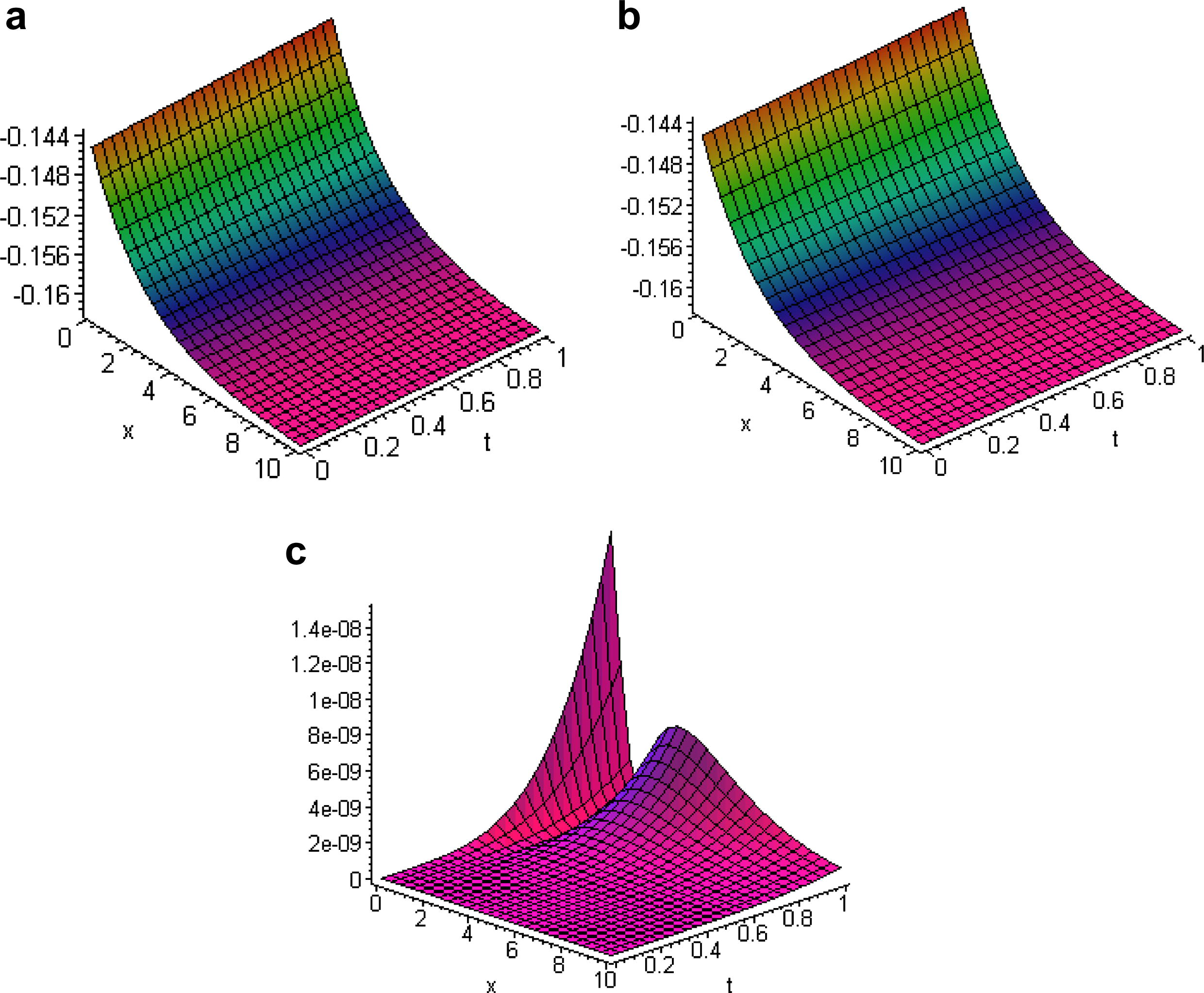
The plot of exact solution (3), the 3th order of approximate solution obtained using the VIM and comparison between the exact and numerical solutions of this example are shown in Fig. 1.
Let us have the following form of Kuramoto–Sivashinsky equation
With initial condition
The solution of the above problem is recognized
For solving by VIM we obtain the recurrence relation
Starting with the initial approximation in (6), the next iterates ‘s will be obtained.
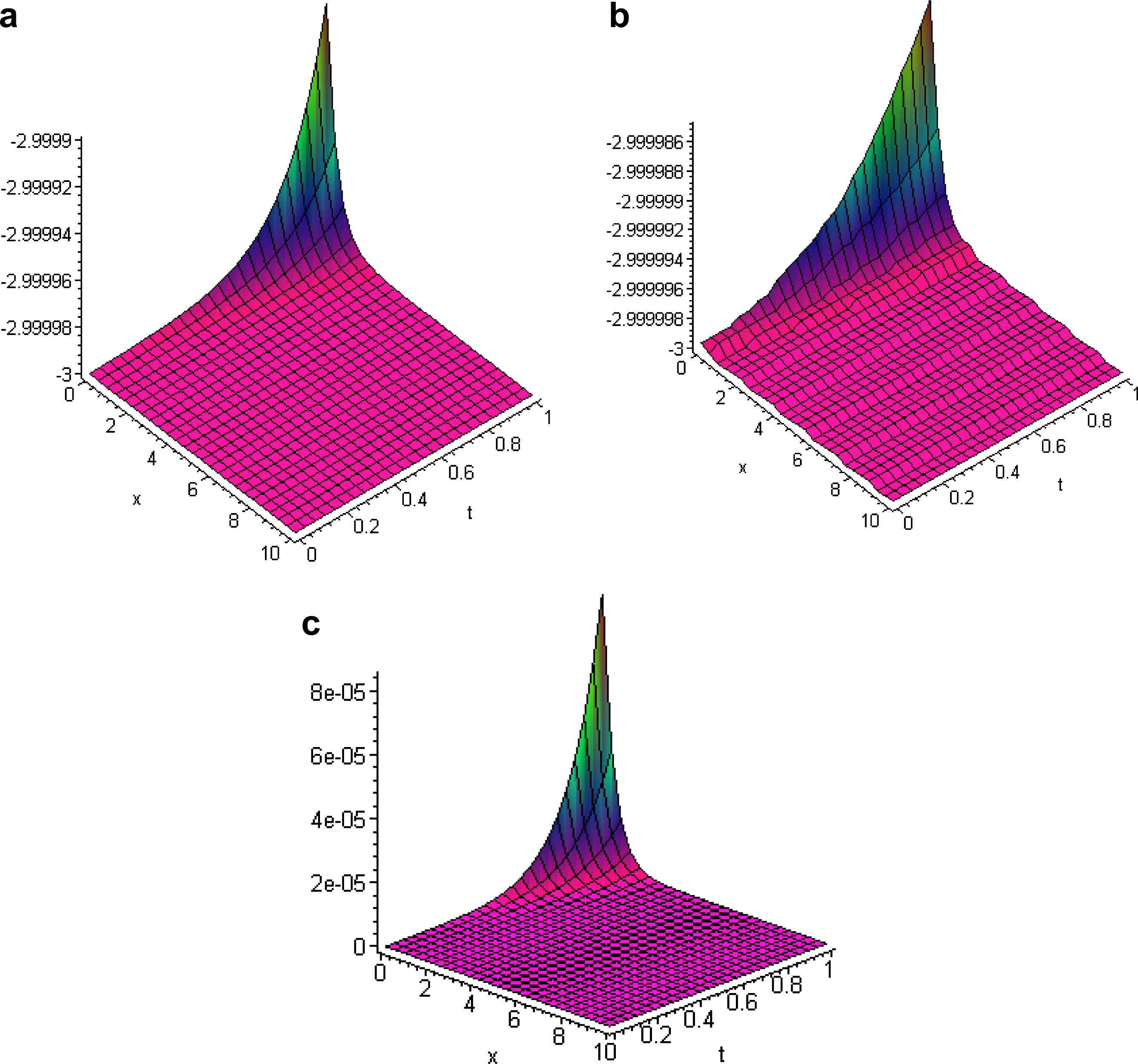
The plot of exact solution (5), the 3th order of approximate solution obtained using the VIM and comparison between the exact and numerical solutions are shown in Fig. 2.
As the last example, we try the case of in (1) as:
Its exact solution of above problem reads
With initial condition
For solving by VIM we obtain the recurrence relation
Using the initial approximation in (8), approximations ‘s will be calculated, successively.
The plot of exact solution (7), the 3th order of approximate solution obtained using the VIM and comparison between the exact and numerical solutions of this example are shown in Fig. 3.

- The surface shows the solution
for Example 1 when
: (a) exact solution (3), (b) 3th order of approximate solution (4) and (c) the absolute error between exact and numerical solutions.
- The surface shows the solution
for Example 2 when
: (a) exact solution (5), (b) 3th order of approximate solution (6) and (c) the absolute error between exact and numerical solutions.
- The surface shows the solution
for Example 3 when
: (a) exact solution (7), (b) 3th order of approximate solution (8) and (c) the absolute error between exact and numerical solutions.
4 Conclusion
In this paper the He's variational iteration method is used to solve the Kuramoto–Sivashinsky equations. We described the method, used it on three test problems, and compared the results with their exact solutions in order to demonstrate the validity and applicability of the method. Moreover, only a small number of iterations are needed to obtain a satisfactory result. The given numerical examples support this claim.
We use the Maple Package to calculate the functions obtained from the variational iteration method
References
- Implicit-explicit BDF methods for the Kuramoto–Sivashinsky equation. Appl. Numer. Math.. 2004;51:151-169.
- [Google Scholar]
- He's variational iteration method for fourth-order parabolic equations. Comput. Math. Appl.. 2007;54:1047-1054.
- [Google Scholar]
- The use of He's variational iteration method for solving the Fokker–Planck equation. Phys. Scr.. 2006;74:310-316.
- [Google Scholar]
- A new approach to nonlinear partial differential equations. Commun. Nonlinear Sci. Numer. Simul.. 1997;2(4):203-205.
- [Google Scholar]
- Variational iteration method for delay differential equations. Commun. Nonlinear Sci. Numer. Simul.. 1997;2(4):235-236.
- [Google Scholar]
- Nonlinear instability at the interface between two viscous fluids. Phys. Fluids. 1985;28:37-54.
- [Google Scholar]
- Persistent propagation of concentration waves in dissipative media far from thermal equilibrium. Pron. Theor. Phys.. 1976;55:356.
- [Google Scholar]
- Second-order splitting combined with orthogonal cubic spline collocation method for the Kuramoto–Sivashinsky equation. Comput. Math. Appl.. 1998;35:5-25.
- [Google Scholar]
- Application of He's variational iteration method and Adomian's decomposition method to the fractional, KdV–Burgers–Kuramoto equation. Comput. Math. Appl.. 2009;58:2091-2097.
- [Google Scholar]
- Instabilities, pattern-formation, and turbulence in flames. Ann. Rev. Fluid Mech.. 1983;15:179-199.
- [Google Scholar]
- Variational iteration method for one dimensional nonlinear thermo elasticity. Chaos, Solitons Fractals. 2007;32:145-149.
- [Google Scholar]
- On the convergence of He's variational iteration method. J. Comput. Appl. Math.. 2007;207:121-128.
- [Google Scholar]
- A mesh-free numerical method for solution of the family of Kuramoto–Sivashinsky equations. Appl. Math. Comput.. 2009;212:458-469.
- [Google Scholar]
- A comparison between the variational iteration method and Adomian decomposition method. J. Comput. Appl. Math.. 2007;207:129-136.
- [Google Scholar]


