

Translate this page into:
Analytical approach to two-dimensional viscous flow with a shrinking sheet via variational iteration algorithm-II
*Corresponding author ahmet.yildirim@ege.edu.tr (Ahmet Yildirim)
-
Received: ,
Accepted: ,
This article was originally published by Elsevier and was migrated to Scientific Scholar after the change of Publisher.
Available online 18 June 2010
Abstract
The purpose of this paper is to employ an analytical approach to a two-dimensional viscous flow with a shrinking sheet. A comparative study of the variational iteration algorithm-II (VIM-II) and the Adomian decomposition method (ADM) are discussed. Both approaches have been applied to obtain the solution of a two-dimensional viscous flow due to a shrinking sheet. This study outlines the significant features of the two methods. Comparison is made with the ADM to highlight the significant features of the VIM-II and its capability of handling completely integrable equations. Through careful investigation of the iteration formulas of the earlier variational iteration algorithm (VIM), we find unnecessary repeated calculations in each iteration. To overcome this shortcoming, we suggest the VIM-II, which has advantages over other iteration formulas, such as the VIM, and the ADM. Further iterations can produce more accurate results and decrease the error.
Keywords
Adomian decomposition method
Padé approximation
Shrinking sheet
Similarity transforms
Variational iteration algorithm-II

1 Introduction
This paper presents a reliable comparison between two recently developed, popular iteration methods, the variational iteration algorithm-II (VIM-II) developed by He et al. (2009) and the Adomian decomposition method (ADM) introduced by Adomian (1988). The use of both methods is common in the literature. The most extensive work carried out on the variational iteration algorithm (VIM) generally is that of He (2000, 2004, 2007, 2008) and He and Lee (2009). Although many researchers have compared the VIM with the ADM, to the best of the authors’ knowledge, no comparison of the VIM-II and the ADM has appeared in the literature thus far. The objectives of this paper are threefold: first, to introduce the advantages of the VIM-II, which primarily lie in its ability to avoid the unnecessary calculations of other iteration methods, namely, the VIM and ADM; second, to illustrate through this comparison that, unlike the widely used ADM, the VIM-II does not require the calculation of Adomian polynomials (Adomian, 1988) for the nonlinear terms that appear in differential equations, as a solution can be obtained without the incorporation of these polynomials; and third, to apply the VIM-II to a fluid mechanics problem, namely, a viscous flow for a shrinking sheet (Fang et al., 2009). An analytical approach is followed to find the numerical value of f″(0), which Wazwaz (2007) has calculated to solve the Blasius equation. This goal is achieved by employing the reliable VIM-II developed by He (2007) and the ADM (Adomian, 1988). For numerical approximation, the resulting series is best manipulated by Padé approximants (Baker, 1975).
2 Padé approximants
Padé approximants constitute the best approximation of a function by a rational function of a given order. Developed by Henri Padé, Padé approximants often provide better approximation of a function than does truncating its Taylor Series, and they may still work in cases in which the Taylor series does not converge. For these reasons, Padé approximants are used extensively in computer calculations, and it is now well known that these approximants have the advantage of being able to manipulate polynomial approximation into the rational functions of polynomials. Through such manipulation, we can gain more information about the mathematical behavior of the solution. In addition, power series are not useful for large values of a variable, say η → ∞, which can be attributed to the possibility of the radius of convergence not being sufficiently large to contain the boundaries of the domain. To provide an effective tool that can handle boundary value problems on an infinite or semi-infinite domain, it is therefore essential to combine the series solution, which is obtained by the iteration method or any other series solution method, with the Padé approximants.
3 Formulation
In this paper, we consider the two basic equations of fluid mechanics in Cartesian coordinates. The continuity equation and momentum equations for viscous flow are
The boundary conditions applicable to the present flow are
For shrinking phenomena, a > 0, a is a shrinking constant, and W is the suction velocity. m = 1 when the sheet shrinks in the x-direction alone, and m = 2 when it shrinks axisymmetrically. We introduce the following similarity transformations.
4 Methods
4.1 He’s variational method
To illustrate the basic concept of He’s VIM, we consider the following general differential equation
where L is a linear operator, N is a nonlinear operator, and g(x) is the source term. According to the VIM, we can construct a correction functional as follows
However, according to the VIM-II, the general form of the algorithm takes the following form
4.2 Adomian decomposition method
A detailed description of the ADM is given in Adomian (1988). Here, we provide only the basic steps as a reminder. Writing Eq. (8) in operator form, we have
Write the general algorithm of Eq. (8) with the initial approximation mentioned in Eq. (14)
The series solution is given by
Padé approximation
f″(0) = α for ADM
f″(0) = α for AVIM
[1/1]
0.292893
0.224748
[2/2]
Complex number
Complex number
[3/3]
Complex number
0.294748
[4/4]
0.247723
0.308086
[5/5]
0.24893
0.249556
The result of VIM and ADM solutions are depicted in Figs. 1 and 2. Fig. 3 compares the two solutions.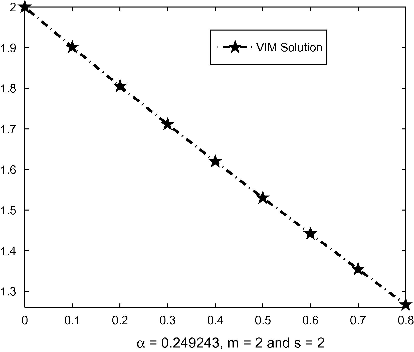
Graphical presentation of VIM solution.
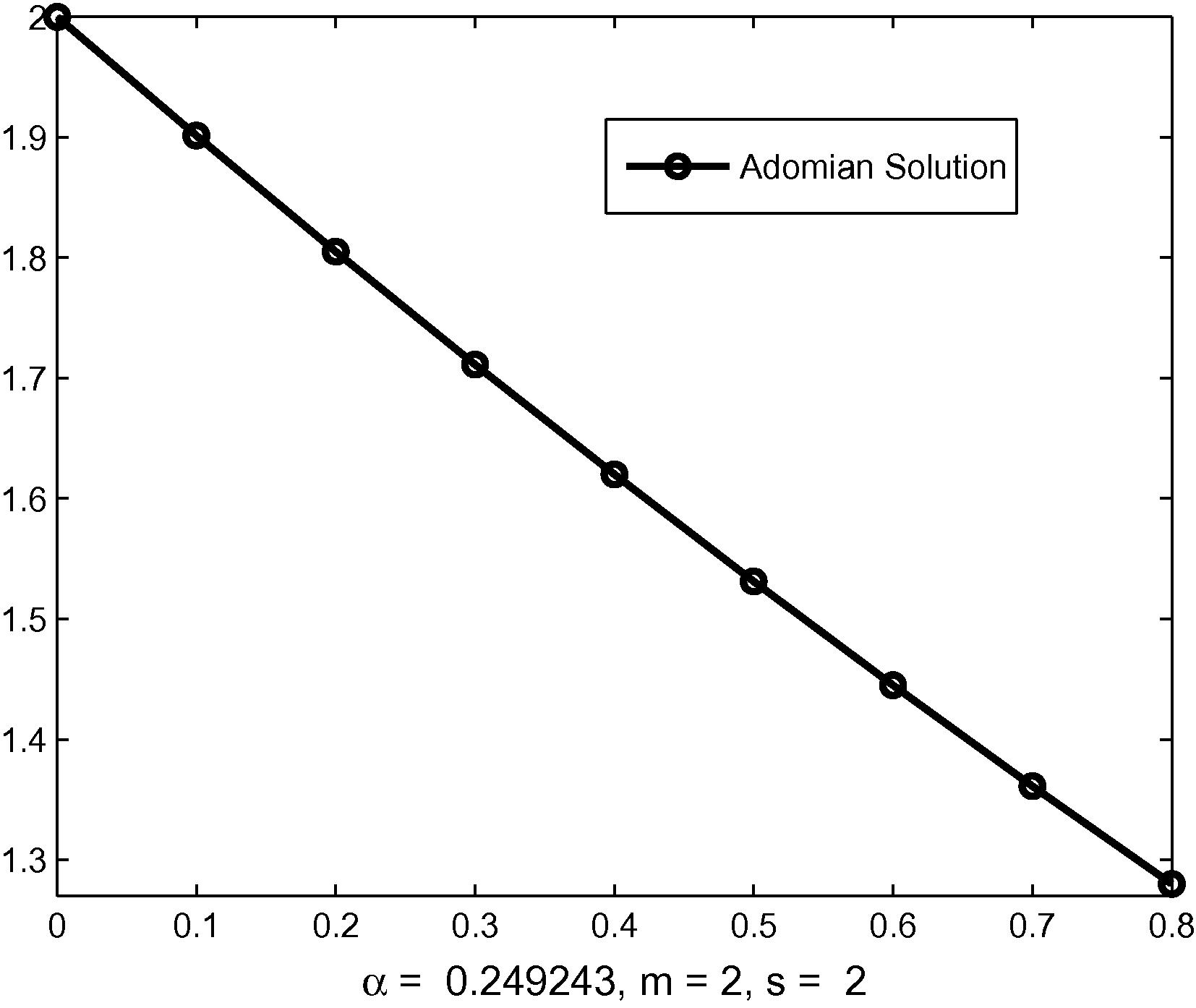
Graphical presentation of Adomian solution.
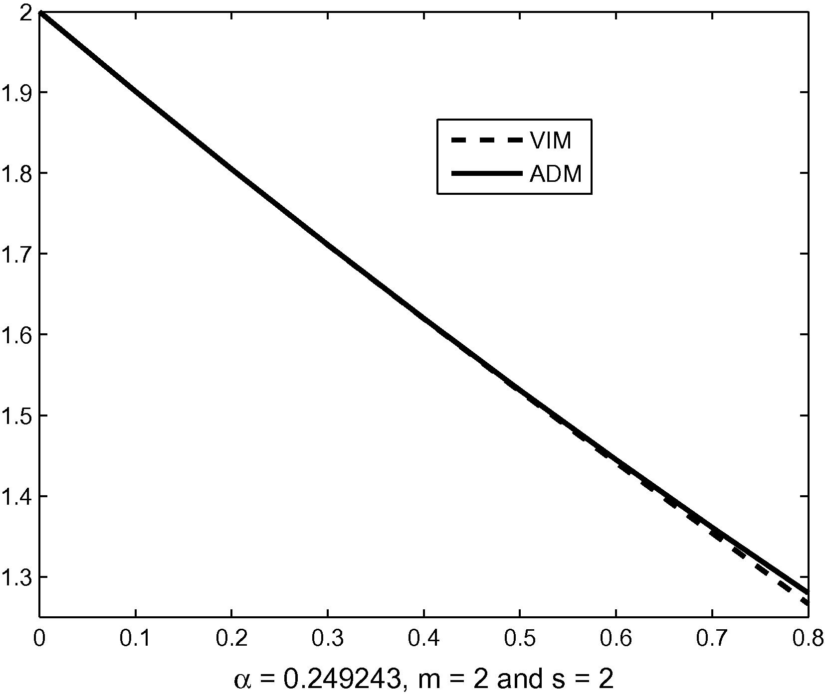
Comparison of the VIM solution and the Adomian solution.
5 Conclusion
This paper presents a variational iteration method, the VIM-II, that can be employed to solve nonlinear differential equations. The method is applied here in a direct manner without the use of linearization, transformation, discretization, perturbation, or restrictive assumptions. The proposed algorithm’s ability to solve nonlinear problems without the use of Adomian polynomials is evidence of its clear advantage over the decomposition method. This study has considered only an axisymmetrically shrinking sheet by taking m = 2.
Acknowledgement
The work described in this paper was fully supported by Modern Textile Institute, Donghua University, 1882 Yan’an Xilu Road, Shanghai 200051, China.
References
- A review of the decomposition method in applied mathematics. J. Math. Anal. Appl.. 1988;135:501-544.
- [Google Scholar]
- Essentials of Padé Approximants. London: Academic Press; 1975.
- Fang, T., Yao, S., Zhang, J., Aziz, A., 2009. Viscous flow over a shrinking sheet with a second order slip flow model. Commun. Nonlinear Sci. Numer. Simul., doi:10.1016/j.cnsns.2009.07.017.
- Variational iteration method for autonomous ordinary differential systems. Appl. Math. Comput.. 2000;114:115-123.
- [Google Scholar]
- Variational principles for some nonlinear partial differential equations with variable coefficients. Chaos Solitions Fract.. 2004;19:847-851.
- [Google Scholar]
- Variational iteration method: some recent results and new interpretations. J. Comput. Appl. Math.. 2007;207:3-17.
- [Google Scholar]
- Erratum to: variational principle for two-dimensional incompressible inviscid flow. Phys. Lett. A. 2008;372:5858-5859.
- [Google Scholar]
- A constrained variational principle for heat conduction. Phys. Lett. A. 2009;373:2614-2615.
- [Google Scholar]
- The variational iteration method which should be followed. Nonlinear Sci. Lett. A. 2009;1:1-30.
- [Google Scholar]
- The variational iteration method for solving two forms of Blasius equation on a half-infinite domain. Appl. Math. Comput.. 2007;188:485-491.
- [Google Scholar]


