

Translate this page into:
Analytic solution to the pendulum equation for a given initial conditions
-
Received: ,
Accepted: ,
This article was originally published by Elsevier and was migrated to Scientific Scholar after the change of Publisher.
Peer review under responsibility of King Saud University.
Abstract
In this paper we give the analytical solution for the undamped pendulum equation for a given arbitrary initial conditions. This solution is expressed in terms of the Jacobian elliptic functions. Approximated trigonometric solution is also provided. Three practical formulas for the period of oscillations are given. The results are illustrated with examples.
Keywords
Undamped pendulum
Duffing equation
Period of oscillations
Jacobian elliptic functions

1 Introduction
The pendulum is a massless rod of lengthlwith a point mass (bob) m at its end (Fig. 1).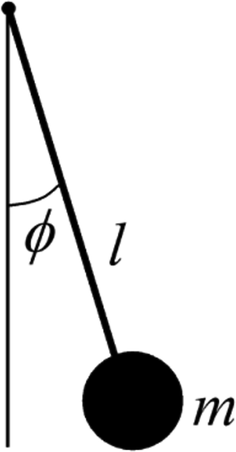
Pendulum.
When the bob performs an angular deflection
from the equilibrium downward position, the force of gravity mg provides a restoring torque
. The rotational form of Newton’s second law of motion states that this torque is equal to the product of the moment of inertia
times the angular acceleration
(Gitterman, 2010),
For small angles,
Eq. (1) reduces to the equation of a harmonic oscillator. Other approximations are
These approximations are compared graphically in Fig. 2.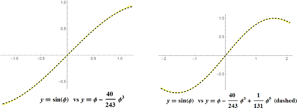
Polynomial approximations to sine function.
2 Analytic Solution to the Pendulum Equation
Our aim is to obtain the solution to the initial value problem
To this end, we make the transformation
Inserting the ansatz (6) into the equation
and taking into account (7) gives
Equating to zero the coefficients of
and
we obtain the system to obtain the system
Solving this system gives
The values of the constants
and
are found from the initial conditions
The general solution to the Duffing equation (Kovacic and Brennan, 2011; Salas and Castillo, 2014) may be expressed in terms of the twelve Jacobian elliptic functions as shown below:
The values of the constants
and
are obtained from the initial conditions
Let
We will make use if the addition formula
Let
Since
We have
Define the residual
To determine the constants
and c we solve the system
Solving system (21) and taking into account (17) we obtain, after some algebraic simplifications, the following expression for the solution to the pendulum Eq. (4):
This solution may also be expressed in the forms
The period of oscillations is given by
This number may be approximated by means of the formulas
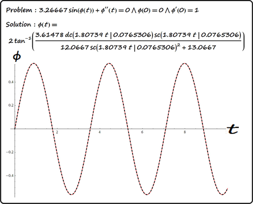
- The dashed curve is that of the numerical solution.
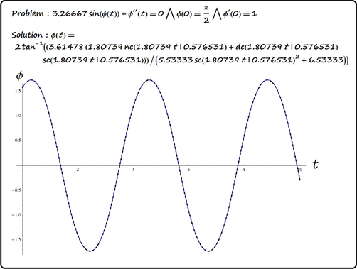
- The dashed curve is that of the numerical solution.
3 Trigonometric approximations
In this section we provide some approximations that solve in a reasonable way the pendulum equation in terms of trigonometric functions. From (3), we see that the equation of the pendulum
may be approximated by means of the equation
Let us consider the case when
Define the residual
as
Direct calculations show that
. In order to find the values of the constants k and
we solve the system
This system reads
A solution is
Compare the exact and approximated trigonometric solution for the pendulum equation
Figs. 5 and 6.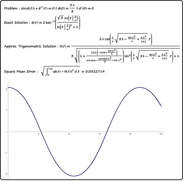
The dashed curve is that of the trigonometric solution.
The dashed curve is that of the trigonometric solution.
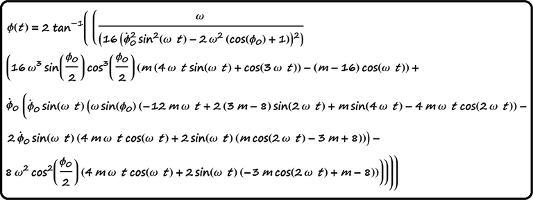
If we are interested in a trigonometric solution to the pendulum equation for a given initial conditions, we may approximate the exact solution by means of trigonometric functions. Let us consider solution given by Eq. (24). The trigonometric approximation is good when the modulus mis a small number. This approximation reads.
Other approximations may be found in Belendez et al. (2012) and Belendez et al. (2016).
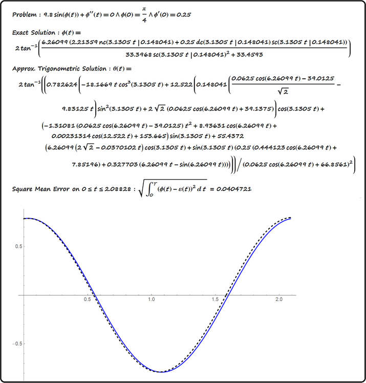
- The dashed curve is that of the trigonometric solution.
4 Conclusions
We have derived the exact solution to the undamped pendulum equation for arbitrary given initial conditions. We conclude that the pendulum equation is closely related to both cubic and cubic-quintic Duffing oscillator equations. Two kinds of trigonometric approximate solutions were provided. We may say that trigonometric approximations are good when the modulus of the Jacobian elliptic functions is a small number say, a number in absolute value less that .The techniques used are applicable for solving the Duffing and the cubic-quintic Duffing equations (Belendez et al., 2012; Belendez et al., 2016) by means of trigonometric ansatze. We think that some of the formulas in this work are new in the literature. Other approaches to nonlinear pendulum may be found in Gitterman (2010), Johannessen (2014) and Salas and Castillo (2014)
References
- Analytical approximate solutions for the cubic-quintic Duffing oscillator in terms of elementary functions. J. Appl. Math., Q3 2012 Article ID 286290,16 pages, ISSN 1110-757X. The special issue Advances in Nonlinear Vibration
- [Google Scholar]
- Exact solution for the unforced Duffing oscillator with cubic and quintic nonlinearities. Nonlinear Dyn. (NODY). 2016;86:1687-1700.
- [Google Scholar]
- Erzwungene schwingungen bei veränderlicher eigenfrequenz und ihre technische bedeutung, Series: Sammlung Vieweg, No 41/42. Braunschweig: Vieweg & Sohn; 1918.
- The Caothic Pendulum. World Scientific Publishing Co., Pte. Ltd.; 2010.
- An analytical solution to the equation of motion for the damped nonlinear pendulum. Eur. J. Phys.. 2014;35:035014
- [Google Scholar]
- The Duffing Equation: Nonlinear Oscillators and their Behaviour (1st ed.). John Wiley & Sons Ltd; 2011.
- Exact solution to duffing equation and the pendulum equation. Appl. Math. Sci.. 2014;8:8781-8789.
- [Google Scholar]


