Analysis of a fractional-order chaotic system in the context of the Caputo fractional derivative via bifurcation and Lyapunov exponents

1 Introduction

Modeling real word problems in fractional calculus continues to interest many authors and researchers. The interpretations of the fractional operators used in the modeling physical problems continue to have many propositions. Nowadays, it is provided that the fractional operators have memories effects role in the modeling physical phenomena (Sene, 2020b), finance (Chen et al., 2014; Gao and Ma, 2009), biological phenomena (Mansal and Sene, 2020; Naik et al., 2020b; Yavuz and Ozdemir, 2020; Yavuz and Bonyah, 2019; Yavuz and Sene, 2020), fundamental mathematics and applications (Mekkaoui et al., 2019; Yavuz, 2019) and many other fields (Naik et al., 2020a). Modeling chaotic systems using fractional operators have been experienced in fractional calculus by Petras (xxxx). For applications of chaos in modeling electrical circuits, see also in Petras (2008), the author finds the fractional operators are interesting tools that can play an important role in the chaos. As we will provide in this paper, the role of the fractional operator in modeling a chaotic system is to obtain various types of chaos for the same system: chaotic behaviors and hyperchaotic behaviors. This conclusion is fundamental because a chaotic system with integer-order derivative can not combine at the same time, the chaotic and hyperchaotic behaviors for an identical system. The varieties of fractional operators in fractional calculus give the importance of this field of mathematics. There exist a fractional derivative operator with Mittag–Leffler function as the derivative introduced in Atangana and Baleanu (2016) by Atangana and Baleanu, the Caputo-Fabrizio derivative proposed by Caputo and Fabrizio (2015), the Caputo derivative, and the Riemann–Liouville derivative, which can be found in Kilbas et al. (2006) and Podlubny (1999). There exist many other fractional operators, many modified operators, and generalization of the fractional operators exist, too, see in Fahd et al. (2017). Known as very sensitive to the variations of the initial conditions, this paper will use the Caputo derivative in modeling a chaotic system. The obtained equation with the fractional operator will be called fractional-order chaotic system.

In terms of a chaotic system, many investigations exist, we give in this paragraph a brief review of the literature. In Rajagopal et al. (2016), the authors have presented works related to brushless DC motor in the context of fractional order derivative. In Ren et al. (2018), the authors have proposed a new hyperjerk chaotic system that has any equilibrium points and finds good results in this type of chaotic system. In Rajagopal et al. (2017), Rajagopal et al. have presented using the fractional-order derivative a hyperchaotic chameleon system. In Vaidyanathan et al. (2014), Vaidyanathan et al. have proposed a 5D novel hyperchaotic system and studied the properties of the proposed system as the detection of chaos, the synchronization, the electrical implementation, and the Lyapunov exponents. In Akgul et al. (2017), Akgul et al. have investigated a 4D wing chaotic system and have proposed its adaptative control and its electrical implementation. In Rajagopal et al. (2019), the authors have proposed a new simple chaotic system with various topological attractors; they have presented in this work the bifurcation diagrams, which are very important in a chaotic system. In Pham et al. (2017), Pham et al. have presented a new chaotic model without equilibrium, have proposed its phase portraits, its bifurcation diagrams by analyzing the small variations of the parameters of the proposed model, and have presented its corresponding Lyapunov exponents. In Vaidyanathan et al. (2014), the authors have investigated an adaptative control to stabilize the possible equilibrium points of a new nine-term chaotic system. In Jafari and Sprott (2013), Jafari and Sprott have presented a simple flow chaotic system which admits a line equilibrium; they have investigated the phase portraits, the Lyapunov exponents for the classification of the types of chaos, and have presented the bifurcation diagrams. In Sprott et al. (2017), Sprott et al. study a megastability for a class of chaotic systems. InLu et al. (2004), Lu et al. have proposed a detailed review and tutorial related to the chaotic systems. For other investigation related to the chaotic systems, see in Shahiri et al. (xxxx), Chen et al. (2014), Xu and He (2013), Wang et al. (2011), Chen (2008), Shaojie et al. (2020), Akgul et al. (xxxx), Rajagopal et al. (2020) and Diouf et al. (2020). For more applications of chaotic systems in the context of fractional operators, see the following papers Solis-Perez et al. (2020), Coronel-Escamilla et al. (2020), Owolabi et al. (2020) and Emmanuel Solis-Perez and Francisco Gomez-Aguilar (2020).

The investigations in this paper are motivated by the memory effect properties and the detection of the chaos, which can be obtained using the fractional operator. The objective of this paper will be to propose a numerical scheme to solve a class of fractional-order chaotic systems. The numerical scheme will be beneficial to obtain the phase portraits of the considered chaotic system. The various phase portraits will inform us there exist a significant influence of the order of the fractional derivative into modeling the chaotic systems. In other words, news natures in the dynamics of the chaotic systems are obtained as the chaotic and hyperchaotic behaviors for the same chaotic system. To detect the chaotic and hyperchaotic behaviors, the Lyapunov exponents will be calculated for the different values of the fractional-order derivative of the considered system. Danca algorithm will be used to arrives at our end In Danca and Kuznetsov (2018). In this paper, we will also analyze using bifurcation diagrams the influence of the parameters of the considered chaotic system in the dynamics. The main novelty in this paper will be the bifurcation diagrams and the Lyapunov exponents of the fractional-order chaotic system. The works presented in this paper can be applied in biology like modeling disease using chaotic systems because many diseases cause many dies in the world, like presently the novel coronavirus. The chaotic system presented in this paper can be used in modeling electrical circuits. Note that the main importance of the chaotic and hyperchaotic system is modeling chaotic electrical circuits and simulations. The chaotic system also plays many roles in modeling financial markets.(Diouf et al., 2020).

This paper is divided into the following forms. In Section 2, we recall the operators used in modeling our chaotic system. In Section 3, we present the fractional-order chaotic system considered in this present work. In Section 4, the numerical scheme used for the phase portraits has been introduced. In Section 5, the phase portraits of the fractional chaotic system for different values of the order of the Caputo derivative are proposed. In this section, the influence of the fractional-order will be observed. In Section 6, the local stability analysis of the trivial equilibrium point will be analyzed using the Matignon criterion. In Section 7, we investigate the variations of the parameters of the fractional-order chaotic system using bifurcation diagrams. In Section 8, we characterize the nature of chaos by calculation the Lyapunov exponents in the context of fractional order derivative. In Section 9, the conclusion and future directions of works have been provided. In other words, we summarize all the main findings in this paper and give future directions for researches.

2 Basic fractional calculus operators

There exist various types of fractional operators in fractional calculus like the Riemann–Liouville derivative (Kilbas et al., 2006; Podlubny, 1999), the Caputo derivative (Kilbas et al., 2006; Podlubny, 1999), the Caputo-Fabrizio derivative (Caputo and Fabrizio, 2015), the Atangana-Baleanu derivative (Atangana and Baleanu, 2016), the conformable derivative, the Hilfer derivative, and many others modifications of the above-cited operators. In modeling chaotic systems, the Caputo derivative is preferred due to its physical meaning, and the memory effect can be observed as well. In this section, we recall the so-called Riemann–Liouville integral, its associated fractional operator, and the Caputo fractional derivative. We have the following definitions.

The other definitions of the fractional operators are not enumerated in this section, but their explicit forms and properties can be found in Atangana and Baleanu (2016) and Caputo and Fabrizio (2015).

3 Fractional-order chaotic system description

Chaotic systems have attracted many researchers due to its many applications in physics and modeling electrical circuits. In this present section, we consider the chaotic system recalled in Lu et al. (2004) and described by the following differential equation with Caputo fractional derivative

4 Numerical scheme for the fractional order chaotic model

This section will be devoted to describing the numerical scheme for the fractional chaotic model proposed in Eqs. (4)–(6). The present numerical scheme uses the analytical solutions and the standard scheme proposed for the Riemann–Liouville fractional integral. In chaotic dynamics, it isn’t easy to obtain the exact solutions due to the nonlinearity of the equations that constitute the system. Therefore many analytical methods as the Laplace transform, the Sodumu transform, the homotopy analysis method, the homotopy perturbation can not be applied satisfactorily. For example, in the case of the Homotopy method, the problem appears on the number of iterations to consider and to have stable and converging solutions. The main alternative to the phases portrait of the chaotic systems is to use the numerical schemes: implicit scheme, explicit scheme, Adams Bashford scheme, and others. As can be observed, the method of discretization used in this paper includes the discretization of the Riemann–Liouville derivative instead of the discretization of the Caputo derivative described in Jannelli (2018). The numerical proposed in this section has many advantages regarding the method previously cited; our method is stable, consistent, and convergent; see in Garrappa (2019) for more pieces of information. In this section, we propose a numerical technique that can be used in the fractional context. The analytical solutions of the fractional-order chaotic system (4)–(6) is defined as the forms

The phase portraits in the next section will be represented using the proposed numerical scheme in this section. The simplicity of the numerical scheme proposed in this section comes from the discretization of the Riemann–Liouville integral, not from the discretization of the Caputo derivative. The second advantage is the stability of the presented numerical scheme comes directly for the existence of the solutions of the considered system. Note that because the Lipschitz continuous of the functions $U,V$ , and W ensure the existence and the uniqueness of the model considered in this paper.

5 Phase portraits related to the fractional order derivative

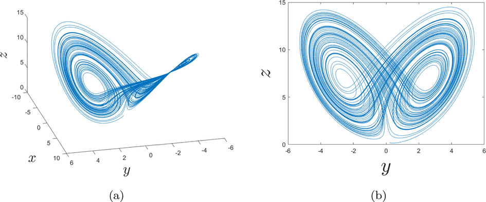
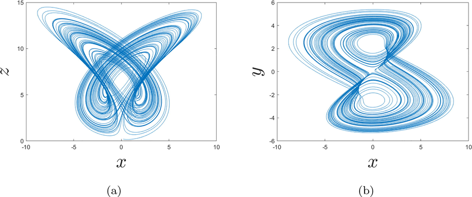
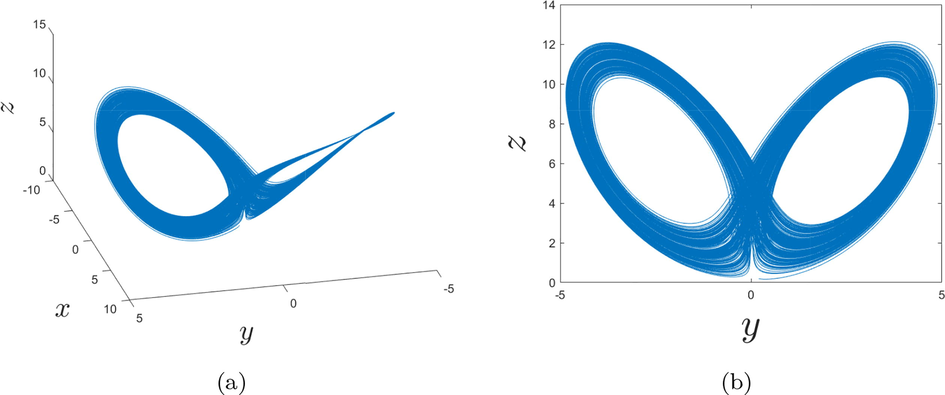
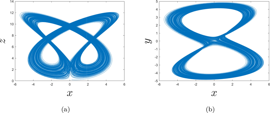
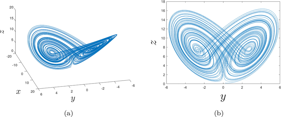
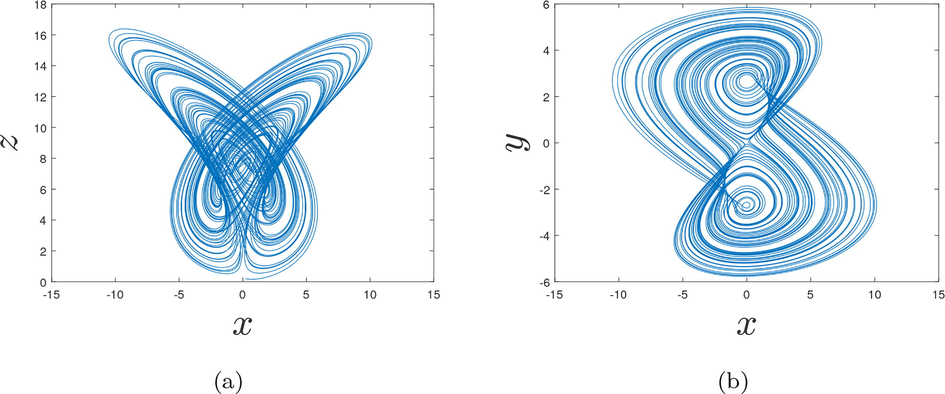
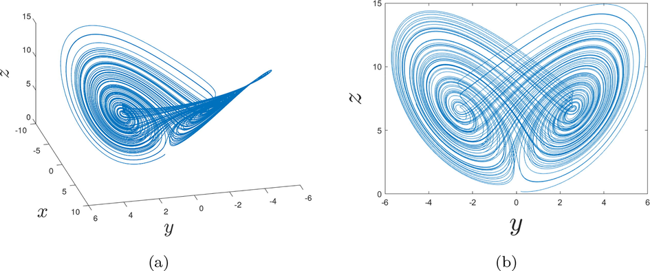
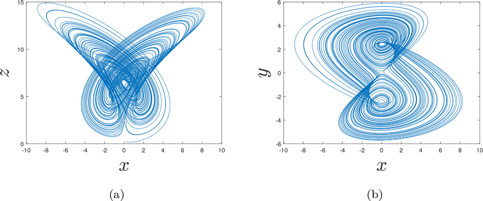
In this section, we represent the phase portraits of the fractional-order chaotic model considering different values of the order of the Caputo derivative by using the numerical discretization used in the previous section. Our objective is to analyze the impact of the fractional-order derivative in the behaviors of the fractional-order chaotic system. We consider in the first graphical representations the order $\alpha =0.94$ . Due to the sensibility of chaos to the initial condition, we take time to recall the initial condition considered in this paper; there are $x(0)=0.2,y(0)=0.2$ , and $z(0)=0.2$ .

In Figs. 1a, b and 2a, b are represented the dynamics of the fractional-order chaotic system in different planes. As we can observe in Figs. 1a, b and 2a, b, at the order $\alpha =0.94$ , we detect the presence of chaos. The main question will be, what is the type of chaos observed at the order $\alpha =0.94$ ? This question will be addressed in the forthcoming section using the Lyapunov exponent.

Close

Fig. 1

Behaviors of the fractional chaotic system for the order $\alpha =0.94$ .

Export to PPT

Close

Fig. 2

Behaviors of the fractional chaotic system for the order $\alpha =0.94$ .

Export to PPT

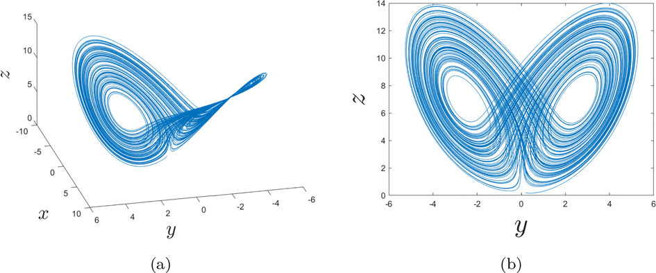
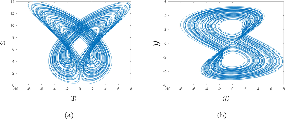
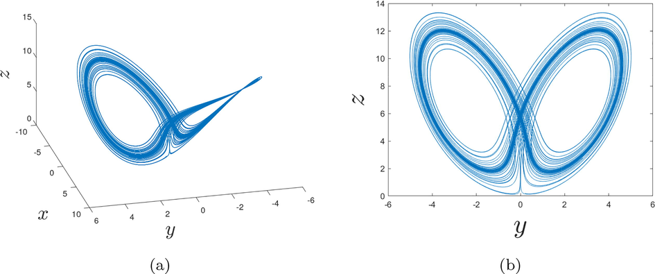
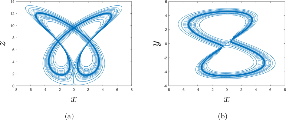
In this present part, we consider the following order $\alpha =0.84$ of the Caputo derivative and depict the phase portraits for our chaotic system. In Figs. 3a, b and 4a, b are represented the dynamics of the fractional-order chaotic system in different planes. As we can observe in Figs. 3a, b and 4a, b, at the order $\alpha =0.84$ , we detect presence of high chaos more than at order $\alpha =0.94$ .The Lyapunov exponent will justify the presence of high chaos in the next section. In terms of comparison, we can observe the fractional-order graphically has a significant impact on the behaviors of the chaotic system considered in this paper. For confirmations of this influence, we represent the next graphics with the order $\alpha =0.64$ .

Close

Fig. 3

Behaviors of the fractional chaotic system for the order $\alpha =0.84$ .

Export to PPT

Close

Fig. 4

Behaviors of the fractional chaotic system for the order $\alpha =0.84$ .

Export to PPT

In Figs. 5a, b and 6a, b are represented the dynamics of the fractional-order chaotic system in different planes.

Close

Fig. 5

Behaviors of the fractional chaotic system for the order $\alpha =0.64$ .

Export to PPT

Close

Fig. 6

Behaviors of the fractional chaotic system for the order $\alpha =0.64$ .

Export to PPT

In all these three cases, how the differences in the behaviors of the dynamics will be shown in the next section. Fractional-order derivative is an excellent compromise to have more complex types of chaos. In our context the chaotic behaviors or hyperchaotic behaviors exist when the Caputo derivative $\alpha$ is into the interval $(0.6,1)$ .

6 Local stability analysis in fractional context

In this section, we focus on the local stability of the equilibrium points of the fractional-order chaotic system considered in this paper. As we know, in chaotic systems in general, the equilibrium points are not stable. This property is one of the main property respected by chaotic systems. We use the standard criterion used in fractional calculus for local stability. The criterion is originated from Matignon, see in Matignon (1996) and Ahmed et al. (2006). For investigations related to stability analysis, see more pieces of information in the following papers (Sene, 2019, 2020a). We first determine the equilibrium points satisfying the following equations

7 Sensibility to the variation of the parameters of the model

This section will be the step to analyze the impact of the variations of the parameters of the considered model. We use so-called bifurcation diagrams. Bifurcation studies the impact generated by the small changes in the parameters of the model. In this section, we set $\alpha =0.94$ with the initial conditions $x(0)=0.2,y(0)=0.2$ , and $z(0)=0.2$ .

Before beginning the study of the variation of the first parameter a, to observe the impact due to the small changes of the parameter a, we depict the phase portraits of the considered fractional-order chaotic system with $a=-2.5,b=-6.4,c=1$ and $d=1$ . In Figs. 7a, b and 8a, b are represented the dynamics of the fractional-order chaotic system in different planes. Considering $a=-2$ and $a=-2.5$ , we observe comparing the Figs. 1a, b, 2a, b and Figs. 7a, b, 8a b, the parameter a has a significant impact on the dynamics of the fractional-order chaotic system. Let’s a small variation of the parameter a, and we conserve the other parameters as $b=-6.4,c=1$ and $d=1$ . The bifurcation diagram versus the parameter a is depicted in the Fig. 9. In Fig. 9, we can observe the chaotic behaviors are more complex at point $a=-2$ than at point $a=-2.5$ . We notice the hyperchaotic behaviors when a is into the interval $(-2.4,2)$ , but at the point $a=-2$ , the behaviors are chaotic. In interval $(-3,-2.4)$ , we have three double-blind bifurcations.

Close

Fig. 7

Behaviors of the fractional chaotic system for the order $\alpha =0.94$ .

Export to PPT

Close

Fig. 8

Behaviors of the fractional chaotic system for the order $\alpha =0.94$ .

Export to PPT

Close

Fig. 9

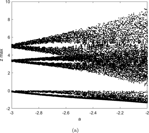
Bifurcation diagram versus small variation of the parameter a.

Export to PPT

Before studying the variation of the second parameter b,we depict the phase portrait of the fractional-order chaotic system with $a=-2,b=-6.4,c=1$ and $d=1$ . In Figs. 10a, b and 11a, b are represented the dynamics of the fractional-order chaotic system in different planes. Considering $b=-6.4$ and $a=-7.4$ , we observe comparing Figs. 1a, b, 2a, b, and Figs. 10a, b, 11a, b, the parameter b has a significant impact on the dynamics of the fractional chaotic system. Let’s a small variation of the parameter b and we conserve the other parameters as $a=-2,c=1$ and $d=1$ . The bifurcation diagram versus the parameter b is depicted in Fig. 12. In Fig. 12, we can observe a small change in the chaotic behaviors at point $a=-7.4$ than at point $a=-6.4$ . The difference is not so significant as it can be observed in Figs. 1a, b, 2a, b, and Figs. 10a, b, 11a, b. We notice chaotic behaviors when a is into the interval $(-7.4,-6.4)$ . Furthermore, in this interval, the chaotic behaviors are very complex.

Close

Fig. 10

Behaviors of the fractional chaotic system for the order $\alpha =0.94$ .

Export to PPT

Close

Fig. 11

Behaviors of the fractional chaotic system for the order $\alpha =0.94$ .

Export to PPT

Close

Fig. 12

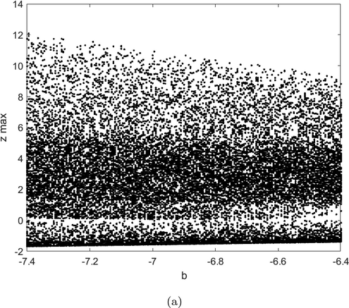
Bifurcation diagram versus small variation of the parameter b.

Export to PPT

Before studying the variation of the parameter c, we depict the phase portraits of the fractional-order chaotic system with $a=-2,b=-6.4$ , and $c=1.5$ . In Figs. 13a, b, and 14a, b are represented the dynamics of the fractional-order chaotic system in different context. Considering $c=1.0$ and $c=1.5$ , we observe comparing Figs. 1a, b, 2a, b, and 10a, b, 11a, b, the parameters c have minor impact in the dynamics of the fractional chaotic system. Let’s a small variation of the parameter c and we conserve the other parameters as $a=-2$ , and $b=-6.4$ . The bifurcation diagram versus the parameter c is depicted in Fig. 15. In Fig. 15, we can observe minor change in the chaotic behaviors at point $c=1$ than at point $c=1.5$ . The minor difference is not so significant as it can be observed in Figs. 1a, b, 2a, b, 13a, b, and 14a, b. We notice chaotic behaviors in all the interval $(1,2)$ when c varies. Furthermore, in this interval, the chaotic behaviors are very complex but do not differs significantly.

Close

Fig. 13

Behaviors of the fractional chaotic system for the order $\alpha =0.94$ .

Export to PPT

Close

Fig. 14

Behaviors of the fractional chaotic system for the order $\alpha =0.94$ .

Export to PPT

Close

Fig. 15

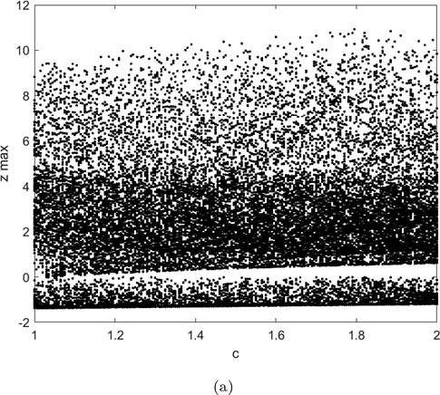
Bifurcation diagram versus small variation of the parameter c.

Export to PPT

8 Chaotic and hyperchaotic detection with Lyapunov exponents

As previously announced in this part, we will justify the nature of the chaos obtained when the orders of the fractional-order derivative vary. We use the Danca algorithm (Danca and Kuznetsov, 2018) and the numerical scheme proposed in our investigations. The values of the Lyapunov exponent versus the time-series variation are represented in the following Table 1 We can remark with the table, at all lines, the sum of the Lyapunov exponents is negative, which corresponds to the dissipativity of the fractional-order chaotic system at order $\alpha =0.94$ . The second remark is that at least two Lyapunov exponents are positive; we can precisely conclude the fractional-order chaotic system at order $\alpha =0.94$ has hyperchaotic behaviors. Note that the value of the Lyapunov exponent represented in Table depend strongly of the considered initial condition in this paper $x(0)=0.2,y(0)=0.2$ , and $z(0)=0.2$ .

In term of comparison, we consider the values of the Lyapunov exponents versus the time-series variation at order $\alpha =0.84$ , see Table 2.

We can observe with the values in the previous table, at all lines, the sum of the Lyapunov exponents is negative, which also corresponds to the dissipativity of the fractional-order chaotic system at order $\alpha =0.84$ . The second remark is that at least two Lyapunov exponents are positive at all lines, we can precisely conclude the fractional chaotic system at order $\alpha =0.84$ has hyperchaotic behaviors. In term of comparison between $\alpha =0.84$ and $\alpha =0.94$ , we can compare the values of $\mathit{LE}1$ in Table 2 and Table 2, we clearly observe the hyperchaotic behaviors are more complex at $\alpha =0.84$ then at order $\alpha =0.84$ . This remark is confirmed by the figures in the phase portraits section.

For the order $\alpha =0.64$ , it is difficult to predict the nature of the chaos, but we note high concentrations of the dynamics of the fractional-order chaotic system. For more analysis, we give in the following table the values of the Lyapunov exponents at the order $\alpha =0.64$ ; we have As it can be confirmed with the Table 3, there exist at time $t=79.98$ under which the hyperchaotic behaviors change to chaotic behaviors. Chaotic because there exist at this step, one positive Lyapunov exponent. The dissipativity of the system is also conserved because the sum of the Lyapunov exponents is at all step negative.

9 Conclusion and futures directions of works

The properties of the fractional-order chaotic system as the phase portraits, the bifurcation diagram, and the Lyapunov exponent have been analyzed. The main result is the Caputo derivative plays a significant role in the nature of the chaos processes. In other words, according to the variations of the values of the Caputo derivative, we can detect with the considered system the chaotic behaviors and the hyperchaotic behaviors. We also find the fractional-order does not impact the local stability of the trivial equilibrium point. The Matignon criterion was used in the stability investigations. The commensurable fractional-order chaotic system has been considered in the present paper; it will be interesting in the future works to investigate the phase portraits, the bifurcation diagram, and the Lyapunov exponent in the context of an incommensurable chaotic system with fractional order derivative. The used derivative can also be changed to see the real impact of the Caputo-Fabrizio derivative and the Atangana-Baleanu derivative in modeling chaotic systems.

Declaration of Competing Interest

The authors declare that they have no known competing financial interests or personal relationships that could have appeared to influence the work reported in this paper.

References

- On some Routh-Hurwitz conditions for fractional order differential equations and their applications in Lorenz, Rossler, Chua and Chen systems. Phys. Lett. A. 2006;358:1-4.
- [Google Scholar]
- Amplitude control analysis of a four-wing chaotic attractor, its electronic circuit designs and microcontroller-based random number generator. J. Circ. Syst. Comput.. 2017;26(12):1750190.
- Akgul, A, Arslan, C., Aricioglu, B. Design of an Interface for Random Number Generators based on Integer and Fractional Order Chaotic Systems. Chaos Theory Appl., 1(1), 1–18.
- New fractional derivatives with nonlocal and non-singular kernel: theory and application to heat transfer model. Thermal Sci.. 2016;20(2):763-769.
- A new definition of fractional derivative without singular kernel. Progr. Fract. Differ. Appl.. 2015;1(2):1-15.
- Nonlinear dynamics and chaos in a fractional-order financial system. Chaos Solitons Fract.. 2008;36:1305-1314.
- Inverse optimal control of hyperchaotic finance system. World J. Model. Simul.. 2014;10(2):83-91.
- Fractional dynamics and synchronization of Kuramoto oscillators with nonlocal, nonsingular and strong memory. Alexandria Eng. J.. 2020;59(4):1941-1952.
- Matlab Code for Lyapunov exponents of fractional-order systems. Int. J. Bifur. Chaos. 2018;28(5):1850067.
- Analysis of the financial chaotic model with the fractional derivative operator. Complexity. 2020;9845031:14.
- [CrossRef] [Google Scholar]
- Novel fractional operators with three orders and power-law, exponential decay and Mittag-Leffler memories involving the truncated M-Derivative. Symmetry. 2020;12(4):626.
- On the generalized fractional derivatives and their Caputo modification. J. Nonlinear Sci. Appl.. 2017;10:2607-2619.
- Numerical solution of fractional differential equations: a survey and a software tutorial. Math.. 2019;6(2):16.
- Simple chaotic flows with a line equilibrium. Chaos Solitons Fract.. 2013;57:79-84.
- Numerical solutions of fractional differential equations arising in engineering sciences. Math.. 2018;8:215.
- Theory and Applications of Fractional Differential Equations, North-Holland Mathematics Studies. Amsterdam, The Netherlands: Elsevier; 2006. p. :204.
- A new chaotic system and beyond: the generalized Lorenz-like system. Int. J. Bifur. Chaos. 2004;14(5):1507-1537.
- Analysis of fractional fishery model with reserve area in the context of time-fractional order derivative. Chaos Solitons Fract.. 2020;140:110200
- Matignon, D., 1996. Stability results on fractional differential equations to control processing. In: Proceedings of the Computational Engineering in Syatems and Application Multiconference; IMACS, IEEE-SMC: Lille, France, 2, 963–968.
- A new approximation scheme for solving ordinary differential equation with Gomez-Atangana-Caputo fractional derivative. Methods Math. Model. 2019:51.
- Chaotic dynamics of a fractional order HIV-1 model involving AIDS-related cancer cells. Chaos Solitons Fract.. 2020;140:110272
- The role of prostitution on HIV transmission with memory: a modeling approach. Alexandria Eng. J.. 2020;59(4):2513-2531.
- Modelling of chaotic processes with caputo fractional order derivative. Entropy. 2020;22(9):1027.
- A note on the fractional-order Chua’s system. Chaos Solitons Fract.. 2008;38:140-147.
- Petras, I. Fractional-Order Chaotic Systems. Nonlinear Physical Science, Springer book, pp. 103–184.
- Coexistence of hidden chaotic attractors in a novel no-equilibrium system. Nonlinear Dyn.. 2017;87:2001-2010.
- Fractional Differential Equations, Mathematics in Science and Engineering. New York, NY, USA: Academic Press; 1999. p. :198.
- A simple chaotic system with topologically different attractors. IEEE Access 2019
- An exponential jerk system, its fractional-order form with dynamical analysis and engineering application. Soft Comput.. 2020;24:7469-7479.
- Dynamic analysis and chaos suppression in a fractional order brushless DC motor. Electr. Eng. 2016
- Hyperchaotic Chameleon: Fractional Order FPGA Implementation. Complexity. 2017;2017
- Ren, S., et al., 2018. A new chaotic flow with hidden attractor: the first hyperjerk system with no equilibrium, Z. Naturforsch., aop, doi: 10.1515/zna-2017-0409.
- Stability analysis of the generalized fractional differential equations with and without exogenous inputs. J. Nonlinear Sci. Appl.. 2019;12:562-572.
- Global asymptotic stability of the fractional differential equations. J. Nonlinear Sci. Appl.. 2020;13:171-175.
- Second-grade fluid model with Caputo-Liouville generalized fractional derivative. Chaos Solitons Fract.. 2020;133:109631
- Shahiri, M.T., et al., Control and synchronization of chaotic fractional-order Coullet System via Active Controller, (2).
- Chaos and complexity in a fractional-order financial system with time delays. Chaos Solitons Fract.. 2020;131:109521
- Chaotic systems and synchronization involving fractional conformable operators of the Riemann-Liouville type. Spec. Funct. Anal. Differ. Equ. 2020:335.
- Megastability: Coexistence of a countable infinity of nested attractors in a periodically-forced oscillator with spatially-periodic damping. Eur. Phys. J. Spec. Top.. 2017;226:1979-1985.
- Hyperchaos, adaptive control and synchronization of a novel 5-D hyperchaotic system with three positive Lyapunov exponents and its SPICE implementation. Arch. Control Sci.. 2014;24(4):409-446.
- Global chaos control of a novel nine-term chaotic system via sliding mode control. Stud. Comput. Intell. 2014:571-590.
- Analysis of nonlinear dynamics and chaos in a fractional order financial system with time delay. Comput. Math. Appl.. 2011;62:1531-1539.
- Synchronization of variable order fractional financial system via active control method. Central Eur. J. Phys. 2013
- Characterization of two different fractional operators without singular kernel. Math. Model. Nat. Phen.. 2019;14(3):302.
- New approaches to the fractional dynamics of schistosomiasis disease model. Physica A: Stat. Mech. Appl.. 2019;525:373-393.
- Analysis of an epidemic spreading model with exponential decay law. Math. Sci. Appl. E-Notes. 2020;8(1):142-154.
- Stability analysis and numerical computation of the fractional predator-prey model with the harvesting rate. Fractal Fract.. 2020;4(3):35.