

Translate this page into:
Analysis of a discrete time fractional-order Vallis system
⁎Corresponding author. mmerdan@gumushane.edu.tr (Mehmet MERDAN)
-
Received: ,
Accepted: ,
This article was originally published by Elsevier and was migrated to Scientific Scholar after the change of Publisher.
Peer review under responsibility of King Saud University.
Abstract
Vallis system is a model describing nonlinear interactions of the atmosphere and temperature fluctuations with a strong influence in the equatorial part of the Pacific Ocean. As the model approaches the fractional order from the integer order, numerical simulations for different situations arise. To see the behavior of the simulations, several cases involving integer analysis with different non-integer values of the Vallis systems were applied. In this work, a fractional mathematical model is constructed using the Caputo derivative. The local asymptotic stability of the equilibrium points of the fractional-order model is obtained from the fundamental production number. The chaotic behavior of this system is studied using the Caputo derivative and Lyapunov stability theory. Hopf bifurcation is used to vary the oscillation of the system in steady and unsteady states. In order to perform these numerical simulations, we apply Grünwald–Letnikov tactics with Binomial coefficients to obtain the effects on the non-integer fractional degree and discrete time vallis system and plot the phase diagrams and phase portraits with the help of MATLAB and MAPLE packages.
Keywords
Caputo derivative
Chaotic behavior
Grünwald–Letnikov algorithm
Vallis system
Equilibrium point
Jury criterion

1 Introduction
Difference equations, which emerged as discretization and numerical solutions of differential equations, are one of the rich branches of mathematics. However, it is known that mathematical models will exhibit complex behaviors have events such as bifurcation and chaotic dynamics. Historically, mathematical models have been used to solve many problems. Mathematical models are used in many places such as difference equations, graph theory, matrices. In the literature, it appears that difference equations are used to model a system related to time. The chaotic behavior that emerges from mathematical models is studied by analyzing the system (Deepika et al., 2023). Chaotic dynamics is a nonlinear deterministic system with a wide variety of dynamic behavior that is sensitive to initial conditions and has orbitals limited to phase fields. The study of the behavior of a nonlinear fractional system is of great interest to many scientists and engineers (Bagley et al., 1991; Das et al., 2017). It becomes more attractive when found in nonlinear fractional-order systems, especially in the chaos phenomenon. Edward N. Lorenz, an American mathematician, discovered the first chaotic attractor. A characteristic of chaos is its sensitivity to initial conditions. Lyapunov methods are a powerful system for analyzing the dynamics of nonlinear fractional-order systems and are used to easily obtain stability analysis (Naik et al., 2023). A new definition, the Caputo fractional derivative, is proposed to avoid the singular point in the calculation of the fractional order derivative (Wang et al., 2014). In the last years, bifurcation theory has been developing by adding new ideas on certain topics of mathematical science (Wang et al., 2018; Rajagopal et al., 2019; Zafar et al., 2020;Talbi et al., 2020;George et al., 2022;Khan et al., 2022;Wang et al., 2022; Vaishwar et al., 2022;Akhtar et al., 2021; Veeresha, 2022).
Vallis in 1986 is the description of temperature fluctuations in the western and eastern parts of the equatorial ocean that have a strong impact on the world's global climate (Merdan, 2013). The Vallis system is a modification of the Lorenz system with p = 0 (Garay et al., 2015).This system proved the existence of chaos and it was shown that the El-Nino event is related to the chaotic behavior of the Vallis system. Alkahtani (Alkahtani et al., 2016) studied the Caputo derivatives and the Vallis model and drew the phase portraits of the proportional fractional Vallis system with this derivative. At each critical point in the bifurcation point, all eigenvalues of the Jacobian matrix are calculated. The fractional-order Vallis system has not been investigated much. Recently (Zafar et al., 2020;Singh et al., 2018; Deshpande et al., 2019; Das et al., 2023). Binomial coefficients on the fractional-order Vallis system and three equilibrium points were obtained using the fractional-order Grünwald-Letnikov method. The results of asymptotic stability of all three equilibrium points are similarity as those calculated in Merdan (Merdan, 2013).
In this paper, the existence of equilibria of the fractional order Vallis system is computed. The fractional order of the discrete-time Vallis system was obtained by using the Caputo method in the model. By applying the Jury criterion to this discrete-time system, the local stability of the equilibria is established. By applying Hopf bifurcation on the Vallis system, it is seen that it is unstable for its right neighborhood on the equilibrium points. Phase portraits and phase diagrams of the Vallis system are drawn with the help of the fractional-order Grünwald-Letnikov technique related to binomial coefficients.
2 Methodology
2.1 Vallis system
In 1986, Vallis was awarded three nonlinear systems for the identification of temperature fluctuations in the western and eastern parts of the equatorial ocean, which have a strong impact on the global climate of the earth (Vallis, 1988; Magnitskii et al., 2007).
Here the speed of water at the apparent surface of the ocean, is and and are the temperature in the western and eastern parts of the sea, a are non-negative constants. This study focuses on the discrete Vallis system and the components of the basic three-component model are defined separately as (Vallis, 1986).
2.1.1 The existence of equilibria of the Vallis system
Van den Driessche and Watmough (Driessche, 2002) define it to obtain the threshold parameter known as the basic reproduction number, denoted by . In this threshold parameter, when the equilibrium point is locally asymptotic stable and when the equilibrium point is unstable.
Equilibrium point of model (1)
Then the equilibrium points and are obtained. Here, using the jacobian matrix, we can write the number using the equilibrium point in (1) as follows:
Hence,
the jacobian matrix of the matrices and at the equilibrium point is, for
and from here is the spectral radius of a matrix which gives .
if and only if the model (1) has an equilibrium point.
Proved. If the model (1) has an equilibrium point, it should provide the following equations:
it is calculated that for (3) there is a unique solution that satisfies:
Obviously, if and only if and ■.
2.1.2 Fractional order of the discrete time Vallis system
Fractional differential equations are used to find better inferences from the models made with integer differential equations. Mathematical models created with fractional order ordinary differential equations give better results than integer order ordinary differential equations. Moreover, accurate models emerge as a result of comparing discrete-time models with continuous-time models. The most commonly used fractional derivatives in the literature are Riemann-Liouville and Caputo fractional derivatives. Although there are many studies on discrete-time difference equations, there are few studies on fractional difference equations. In this study, Caputo fractional derivative is used as fractional derivative.
Definition. Caputo, the fractional integral of the function at the level of and , the fractional derivative of defines , where the operator is called the -order Caputo operator (Caputo, 1967).
From the Caputo definition, the initial conditions of the function
with
are made more convenient than the Riemann–Lioville derivative. The fractional-order form of the system (1) is constructed as follows.
Where
represents the caputo fractional derivative. if
,
provides
Let
for any
. Using El-Sayed and Salman's (El-Sayed et al., 2013) discretization method, let's discretize the model (5) as follows:
Where the parameter is the number of steps and the initial conditions are
2.2 Stability of the Vallis system
In this section, the stability conditions of the equilibrium points of the model (6) will be calculated. Let us consider an
-dimensional nonlinear discrete-time system of equations:
Here, are independent parameters and are variables.
Let the characteristic polynomial of (7) at some steady state
has the form
is. Let's determine the stability of the equilibrium state by following the theorem (Li et al., 2011).
(7) for the equilibrium state of the system, let be the parameter value (Galor, 2007; Abdelaziz et al., 2020),
-
If all the eigenvalues of the Jacobian matrix of (7) lie in the open unit disk, i.e. for all , then is asymptotically stable.
-
If the matrix has at least one eigenvalue outside the open unit disk, i.e. | | > 1, then is unstable.
(Schur-Cohn criterion). All roots of the characteristic polynomial F are contained within the unit open disk if and only if (Li et al., 2011):
-
and
-
(when is even) or
(when is odd) or.
(Jury criterion). All the roots of are if and only if in the following cases in the open volume disk (Li et al., 2011):
Here,
in addition, the following Lemma is also mentioned.
Accordingly, for the model (6), to obtain the Jacobian matrix around any point
is done as follows:
Then the eigenvalues of become and .
If and have the following properties.
-
is called a sinking point and if min
-
is called a source point and if max
-
is saddle min
-
is non-hyperbolic if or or where .
Proof If , then the model (6) is seen to have . The Jacobian matrix in is.
(i)-(iv) results are obtained by applying stability conditions using Luo. To discuss the local stability of the equilibrium point we need to calculate the jacobian matrices and as follows.
Let's consider it as follows:
Let's write the characteristic equation of
Where
and .
According to theorem 2, the roots of the equation (11) are with respect to the unit disk if and only if
and equilibrium points are locally asymptotically stable if and min .
and.
. Otherwise is unstable.
Proof if we substitute (12) for (13),
According to the Jury criterion, the model is asymptotically stable when (6), (14a)-(14d) are arranged. It can be concluded that for positive parameters
is positive. Thus, if
(14a) is held. From (14b)-(14d) inequalities, let us consider the following equations:
Equation (15a) has a real root and a double conjugate complex root with the negative coefficient of and . Therefore, when the inequality (14a) is provided. By solving the equation (15b), these four real roots and a pair of conjugate complex roots are obtained. The four real roots are repeated three roots at and the fourth at . Therefore, the interval of the solution is at (14c). When equation (15c) is by solving, (14d) is violated. Therefore, the fact that (14a)-(14d) has at least one solution is obtained from the intersection of , i.e. min .
2.3 Hopf bifurcation
In this section, we will briefly review the discrete Hopf bifurcation criterion. First, let's consider a two-dimensional parameterized system:
For a real variable parameter
and an equilibrium point
, simultaneously
and
is the
value that provides. With the eigenvalues
providing
becomes a Jacobian matrix
in this equilibrium. Also for some small details,
Then the system undergoes a Hopf bifurcation at the bifurcation point . More precisely, for any left neighbor (i.e. , is a constant focus, and for any right neighbor of (i.e. ) this usually changes to be unstable surrounded by a limit cycle (Chen et al., 1999).
2.4 Grünwald-Letnikov algorithm (Binomial coefficients)
Equation obtained from the Grünwald-Letnikov limitation is used. The Grünwald-Letnikov derivative is a generalization of fractional orders of the higher-order derivative, the classical motivation of the derivative is that, from considering the limit form of the nth-order derivative, its similarity to the binomial theorem is seen, and a generalization is obtained in a similar way (Diaz et al., 1974). To study the behavior of a fractional-order chaotic system, the time approximation method GL is used. It has been found that nonlinearity has a great influence on the dynamics of the system. The Grünwald-Letnikov approximation is known that the two constraints are equivalent to the Grünwald-Letnikov constraint and the Caputo constraint. The
node is associated for the numerical
Here K is “memory length”, calculation of time step and binomial shape of is . Let's calculate using the following expression (Vinagre et al., 2003):
Let's consider a nonlinear fractional system:
The initial values with are .
Here, , stands for the derivative of the order of the function, and indicate the limits of the operation.
In this article, the fractional discrete-time equation using the fractional Caputo derivative with and is discussed.
If the Grünwald-Letnikov approach is applied to the equation (19) given above, binomial coefficients are preferred using the concept of memory, and a discrete equation is formed which is shortened by the length of memory.
this relationship (20) can be written as:
This relationship of GL is clear from (21). What is given in this relation is related to the total memory. If we substitute the first equation (20) in system (2), then
If it is written this way,
Since ,
If it is written this way,
Similarly, if the second and third equations of the system (2) are made, Here, using binomial coefficients with GL,
is obtained.
3 Results and discussion
The Runge–Kutta method (fourth order) has been used for solving the system of system (3) and obtains the time series of system variables
and
. The bifurcation diagram in
space is shown in Fig. 1. Here, the maximum Lyapunov exponent corresponding to Fig. 1 is seen to be stable for the fixed point
. The phase portrait of system (3) with
corresponding to different values of
is shown in Fig. 2. Figs. 3 and 4 respectively show the numerical simulation results for
and
based on the Grünwald- Letnikov approach, described in Section 2.4. For
, the fractional-order Chen system with parameter
is chaotic and for
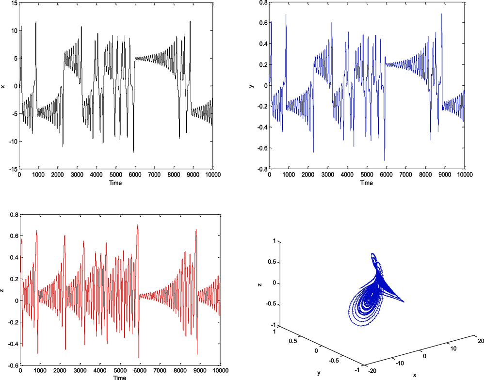
is not. The system (5) is calculated numerically against
. Fig. 5 showed the phase diagram with
, respectively. It was found that when
, system (5) show chaotic behavior. When
and
, chaotic attractors are found
and
phase diagrams are shown in Fig. 5. When
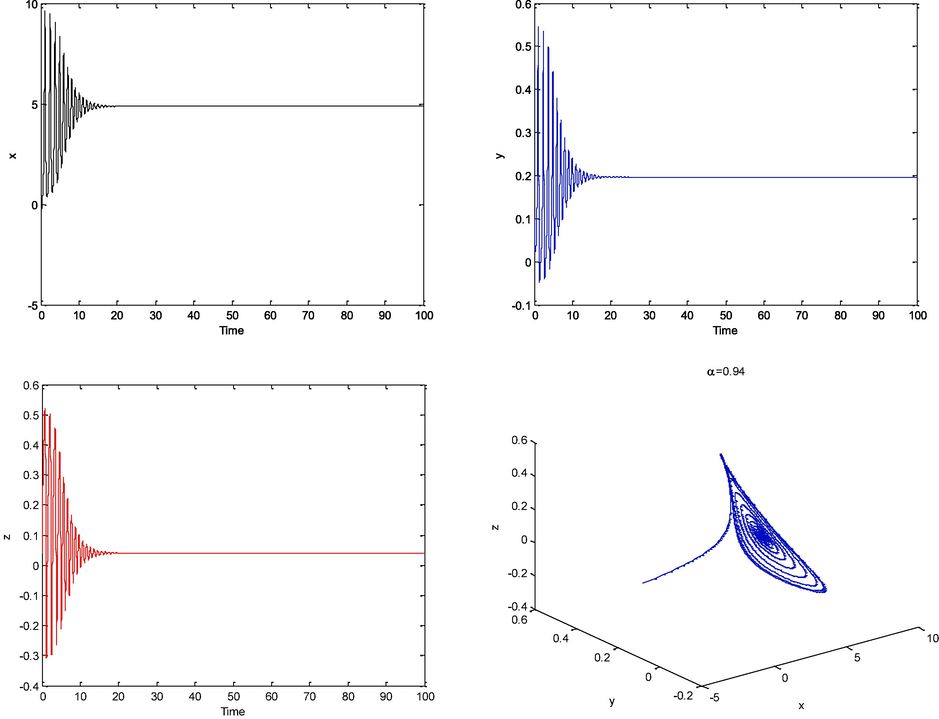
, chaotic motion disappears and the system is stabilized to a fixed point, as shown by the
and
phase plots in Fig. 5 (a3)-(c3). It is obvious that the trajectory for
is attracted to a fixed point. Numerical results obtained from in Fig. 5 indicate the presence of 2- scroll chaotic attractor. System (5) is obtained by numerical solution using Grünwald- Letnikov approach against
. It is explicit in Fig. 6 (d1)-(f1) that system (5) displays chaotic motion. The periodic motion and a fixed point are also plotted in Fig. 6 (e1)-(f4), respectively.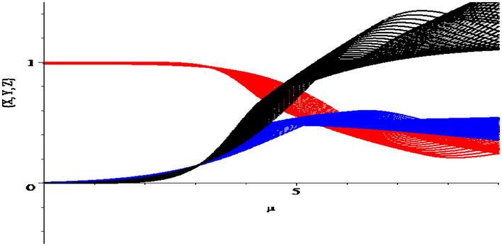
Bifurcation of the discrete-time Vallis model
(Rajagopal et al., 2020).
![Phase portraits of the fractional Vallis system for different values and time interval [0,100] with μ = 170 , h = 0.01 (Zafar et al., 2020).](/content/185/2024/36/2/img/10.1016_j.jksus.2023.103013-fig2.png)
Phase portraits of the fractional Vallis system for different values and time interval [0,100] with
(Zafar et al., 2020).
Phase trajectories of the system (3)
(Zafar et al., 2020).
Phase trajectories of the system (3)
(Zafar et al., 2020).
![System (5) for μ = 170 (a1)-(c1) for α = 1 , (a2)-(c2) for α = 0.99 , (a3)-(c3) for α = 0.94 , (a4)-(c4) for α = 0.90 , tspan[0,100] with phase diagram (Zafar et al., 2020).](/content/185/2024/36/2/img/10.1016_j.jksus.2023.103013-fig5.png)
System (5) for
(a1)-(c1) for
, (a2)-(c2) for
(a3)-(c3) for
, (a4)-(c4) for
, tspan[0,100] with phase diagram (Zafar et al., 2020).
![System (5) for μ = 124.1 (d1)-(f1) for α = 0.99 , (d2)-(f2) for α = 0.98 , (d3)-(f3) for α = 0.97 , (d4)-(f4) for α = 0.96 , tspan[0,100] with phase diagram (Zafar et al., 2020).](/content/185/2024/36/2/img/10.1016_j.jksus.2023.103013-fig6.png)
System (5) for
(d1)-(f1) for
, (d2)-(f2) for
(d3)-(f3) for
, (d4)-(f4) for
, tspan[0,100] with phase diagram (Zafar et al., 2020).
4 Conclusion
In this paper, by discretizing the fractional-order Vallis system is studied. The equilibrium existence of this system is obtained by the number The local asymptotic stability analysis of the three equilibrium points obtained was analyzed by the Jurry criterion. The model undergoes a bifurcation when q increases when the value of μ decreases from a certain threshold values. The hopf bifurcation of the Vallis system was plotted using the values of . By giving the values of to this system, the phase portrait was drawn using the Grendwald-Letnikov algorithm using the values of the diagram.
Acknowledgment
The authors are grateful to referees for careful reading, suggestions, and valuable comments, which have substantially improved the paper.
Declaration of competing interest
The authors declare that they have no known competing financial interests or personal relationships that could have appeared to influence the work reported in this paper.
References
- Codimension one and two bifurcations of a discrete-time fractional-order SEIR measles epidemic model with constan vaccination. Chaos Solit. Fractals. 2020;140:110104
- [CrossRef] [Google Scholar]
- Stability, bifurcation and chaos control of a discretized Leslie prey-predator model, Chaos. Solitons and Fractals. 2021;152:111345
- [CrossRef] [Google Scholar]
- Chaos on the Vallis model for El Nino with fractional operators. Entropy. 2016;18(4):100.
- [CrossRef] [Google Scholar]
- Fractional order state equations for the control of viscoelastically damped structures. J. Guid. Contr. Dyn.. 1991;14(2):304-311.
- [CrossRef] [Google Scholar]
- Linear models of dissipation whose Q is almost frequency independent II. Geophys. J. R. Astrı-on Soc.. 1967;13:529-539.
- [CrossRef] [Google Scholar]
- Controlling Hopf bifurcations: discrete-time systems. Discret. Dyn. Nat. Soc.. 1999;5:29-33.
- [CrossRef] [Google Scholar]
- Stability analysis, chaos control of fractional order Vallis and El-Nino systems and their synchronization. Eee/Caa J. Automat. Sın.. 2017;4(1)
- [CrossRef] [Google Scholar]
- Chaotic dynamics of recharge–discharge El-Nĩno–Southern Oscillation (ENSO) model. Eur. Phys. J. Specıal Top.. 2023;232:217-230.
- [CrossRef] [Google Scholar]
- Dynamics of chaotic waterwheel model with the asymmetric flow within the frame of Caputo fractional operatör. Chaos Solit. Fractals. 2023;169
- [CrossRef] [Google Scholar]
- Chaotic Dynamics of fractional vallis system for El-Nino. Fract. Calc. Appl. 2019
- [CrossRef] [Google Scholar]
- Reproduction numbers and sub-threshold endemic equilibria for compartmental models of disease transmission. Math Biosci.. 2002;180(1):29-48.
- [CrossRef] [Google Scholar]
- Fractional-order Chua’s system: discretization, bifurcation and chaos. In: Advances in difference equations. Vol vol. 13. Springer; 2013.
- [CrossRef] [Google Scholar]
- Galor, O., 2007. Discrete dynamical systems. Springer, Berlin.
- Chaos in Vallis’ asymmetric Lorenz model for El Niño. Chaos Solit. Fractals. 2015;75:253-262.
- [CrossRef] [Google Scholar]
- Bifurcations analysis of a discrete time SIR epidemic model with nonlinear incidence function. Results Phys.. 2022;38:105580
- [CrossRef] [Google Scholar]
- Global dynamics, Neimark-Sacker bifurcation and hybrid control in a Leslie’s prey-predator model. Alex. Eng. J.. 2022;61:11391-11404.
- [CrossRef] [Google Scholar]
- Stability analysis for discrete biological models using algebraic methods. Math. Comput. Sci.. 2011;5:247-262.
- [CrossRef] [Google Scholar]
- Transition to chaos in nonlinear dynamical systems described by ordinary differential equations. Comput. Math. Model.. 2007;18(2)
- [CrossRef] [Google Scholar]
- Numerical solution of the fractional-order Vallis systems using multi-step differential transformation method. App. Math. Model.. 2013;37:6025-6036.
- [CrossRef] [Google Scholar]
- Design of a fractional-order atmospheric model via a class of ACT-like chaotic system and its sliding mode chaos control. Chaos. 2023;33:023129
- [CrossRef] [Google Scholar]
- Taming of the Hopf bifurcation in a driven El Niño model. De Gruyter. 2020;75(8a):699-704.
- [CrossRef] [Google Scholar]
- Antimonotonicity, Bifurcation and Multistability in the Vallis Model for El Nino. Int. J. Bifurcation Chaos. 2019;29(3):1950032.
- [CrossRef] [Google Scholar]
- Singh, P.P., Kumar, V., Tiwari, E., Chauhan, V.K., 2018. Hybrid synchronisation of vallis chaotic systems using nonlinear active control, International Journal of Engineering & Technology, 7 (2.21), 50-52.
- Different dimensional fractional-order discrete chaotic systems based on the Caputo h-difference discrete operator: dynamics, control, and synchronization. Adv. Diff. Eq.. 2020;624
- [CrossRef] [Google Scholar]
- Stability and Hopf-bifurcation analysis of four dimensional minimal neural network model with multiple time delays. Chin. J. Phys.. 2022;77:300-318.
- [CrossRef] [Google Scholar]
- Vallis, G.K., 1986. Chaotic dynamical system. Science 232, 243–1224.
- Conceptual models of El Nino/Southern oscillations. J. Geophys. Res.. 1988;93:13979-13991.
- [CrossRef] [Google Scholar]
- The efficient fractional order based approach to analyze chemical reaction associated with pattern formation. Chaos Solit. Fractals. 2022;165(2)
- [CrossRef] [Google Scholar]
- Petras, I. Two direct Tustin discretization methods for fractional-order differentiator/ integrator. J. Franklin Inst.. 2003;340(5):349-362.
- [CrossRef] [Google Scholar]
- Constructing discrete chaotic systems with positive Lyapunov exponents. Int. J. Bifurcation Chaos. 2018;28(7):1850084.
- [CrossRef] [Google Scholar]
- Hopf bifurcation and chaos of tumor-Lymphatic model with two time delays. Chaos Solit. Fractals. 2022;157:111922
- [CrossRef] [Google Scholar]
- Stability analysis for nonlinear fractional-order systems based on comparison principle. Nonlinear Dyn.. 2014;75:387-402.
- [CrossRef] [Google Scholar]
- Thounthong, P., Tunc, C. Analysis and numerical simulations of fractional order Vallis system. Alexandria Eng. J.. 2020;59:2591-2605.
- [CrossRef] [Google Scholar]


