Translate this page into:
An integrated approach for optimal rail transit corridor identification and scheduling using geographical information system
*Corresponding author at: Department of Civil Engineering, Indian Institute of Science (IISc), Bangalore 560012, Karnataka, India. Tel./fax: +91 80 2293 2329 ashishv@civil.iisc.ernet.in (Ashish Verma), rsashu@yahoo.com (Ashish Verma),
-
Received: ,
Accepted: ,
This article was originally published by Elsevier and was migrated to Scientific Scholar after the change of Publisher.
Available online 15 February 2011
Abstract
In this work an integrated approach has been proposed to identify and schedule a rail transit corridor in a city which has a potential demand for a new rail based mass transit system besides the street transit system and existing rail-based system (if any). The motivation for the present study comes from the present Indian context where, because of recent initiatives of Central Urban Development Ministry, many Urban Local Bodies (ULBs) and transit agencies need to master plan new rail based systems in an optimum way and at the same time attempting to integrate them with other existing public transport (PT) modes. While aligning the new rail transit system, the primary focus of the integrated approach is to optimize the origin–destination (O–D) travel time of the user and at the same time attempting to minimize the operators’ cost. The proposed rail corridor identification model consists of three stages: public transport demand forecasting, creation of corridor link set, and optimization of rail corridor using Geographical Information System (GIS). The objective function for train scheduling model is fixed as minimization of sum of operating cost of trains (operator cost) and total waiting time cost of passengers boarding the train (user costs) subject to load factor and waiting time constraints. The dwell time of train at stations, which is usually considered constant, has been taken as a variable which depends on the actual number of passengers boarding and alighting the train. The model is applied on Thane municipal corporation (TMC) area, a major urban center of the Mumbai metropolitan region (MMR), India. The maximum peak hour ridership obtained on the identified corridor was found to be ideal for recommending light-rail transit system (LRT). The successful application of the model shows the capability of proposed model for a typical Indian city, which has potential demand for a new rail system.
Keywords
Rail transportation
Train scheduling
Public transportation
Geographic information systems
Transportation corridors
Transportation planning
Optimization
Integrated systems
India
1 Introduction
During the second half of last century, urban population in India had grown enormously. This has resulted in a steady increase in number of cities with a population of one million and above from 5 in 1951 to 35 in 2001. This level of urbanization has brought in its wake its own problems, especially with regard to its impact on the infrastructure facilities. The urban transportation systems have come under heavy strain affecting the quality of life of urban dwellers. Lack of mass transportation facilities has resulted in heavy shift of commuter patronage to private and intermediate transport (leading to an imbalance in the modal spilt) and consequently, a huge increase in number of intermediate and private vehicle ownership. Encouraging optimal use of existing and proposed public transport will be an effective way of achieving the desired modal share between different modes. However, an integrated approach toward public transport planning is very essential to achieve this. Then only a public transport system can be made attractive, in terms of quicker travel, convenience, and comfort, to the user. This will also increase the efficiency of each public transport mode available, as they will act as complimentary to each other instead of competing (Verma and Dhingra, 2005).
These present requirements have prompted the concerned agency in India (Ministry of Urban Development, Government of India) to take some drastic steps in the recent past, the prominent among which is the release of National Urban Transport Policy (NUTP) document in 2006, which focuses on “moving people rather than vehicle”. Keeping the NUTP document in perspective, the ministry subsequently launched Jawaharlal Nehru National Urban Renewal Mission (JnNURM) in 63 major Indian cities to fund urban renewal projects at an expected total budget of Indian Rupees (Rs.) 1000 billion (with major share of urban transport). As an important outcome of these efforts a number of Indian cities are currently planning/implementing urban metro rail and BRT systems. This has prompted many Urban Local Bodies (ULBs) and transit agencies to master plan these new BRTS or metro systems in a supposedly optimum way and at the same time attempting to integrate them with other existing public transport (PT) modes. This has resulted in an urgent requirement for developing an innovative methodology for master planning integrated public transport systems, within the existing conditions of Indian cities. The motivation for the present study comes from this very important requirement in the present Indian context. The next section reviews the similar studies done in the past and their drawbacks.
2 Past studies on rail corridor identification and scheduling
In the past, many researchers have developed different approaches to identify rail corridors. Gordon and Willson (1984) examined the prediction of demand for an international cross-section of light-rail transit systems. Simple regression relationships were established between the transit demand in terms of passenger-km and variables like characteristics of transport system, city and population attributes. The drawback with this model is that simple attributes were chosen to depict the variables, which may affect the accuracy of the results. In the study carried out by Clark and Oxley (1991), the rail transit corridors were identified by assigning an origin–destination (O–D) matrix to an assumed spider network. The drawback with the spider network is that it only gives travel desires between different zones and does not give the actual system alignment. Liu et al. (1996) developed a model that determines the optimal location and length of rail lines along a cross-town transportation corridor with the objective of minimizing total transportation costs. This is a relatively simple case of a line-haul corridor, the complexities increase manifold when the rail corridor is to be identified in the context of an integrated mass transit network, which will consist of a network of feeder bus routes for each rail station. Besides this, factors like reasonable inter-station spacing and environmental impacts are not taken into account in this model.
Moorthy (1997) adopted an approach similar to Clark and Oxley (1991), but in addition to spider network, flows were assigned to a combined network of highway and track guided systems and corridors were obtained based on assigned flows. Gipps et al. (2001) identified corridors for a new road or railway using convergence of geospatial imaging, softcopy photogrammetry, regional significance analysis, and alignment optimization. They obtained the corridors based on land availability and cost considerations, which could be suitable for identifying road corridors. However, consideration of actual travel demand pattern of the city is also required for identifying rail corridors. Besides the limitations listed above, all these approaches did not address the need for an integrated planning, i.e., operational, institutional and physical integration, to achieve the forecasted demand for the new rail system, which is very important from the operator’s point of view. This is also important for a choice rider, who will shift to a new public transport only if it offers a comparable level of service. These points have been addressed to some extent in the work carried out by Chien and Schonfeld (1998). They tried to minimize the total cost (supplier plus user cost) of the integrated bus and rail network with an efficient iterative method that successively substitutes variable values obtained through classical analytic optimization. The drawback with their approach was that they used a pre-determined hypothetical network of one rail corridor and perpendicular feeder routes at equal spacing, which may not offer a realistic view.
In another approach by Jha et al. (2007), genetic algorithm and GIS were used for rail line optimization. Two types of costs were formulated and evaluated in the model: operator cost and user cost. Operator cost consists of track related construction cost, station construction cost, right of way cost, earth cost and rail operating cost, whereas user cost consists of access cost, riding time cost and wait cost. Most of these approaches for rail corridor identification did not address the need for an integrated planning for achieving the desired objectives, and also to achieve the forecasted demand for the new rail system.
Verma and Dhingra (2005) proposed a heuristic algorithm for identifying demand oriented urban rail transit corridor on a city using Geographical Information System (GIS) tools. The GIS software TransCAD and GIS Developer’s Kit (GISDK) were used to apply on the model. The objective of the model was to identify the new rail corridor, which is optimum from both users’ and operators’ point of view, however, some of the important variables like; access/egress time, construction cost, etc. were not considered while optimizing the rail corridor alignment. Moreover, the approach used heuristic rules, and was sequential in nature with no iterative mechanism. All these considerations may result in solutions that are sub-optimal. The present work is primarily an attempt to improve upon the previous work of Verma and Dhingra (2005), and focuses on an integrated approach for identifying a rail transit corridor so as to optimize the Origin–Destination (O–D) travel time of the user, which is the total passenger’s travel time from his point of origin (O) to his point of destination (D); and at the same time attempting to minimize the operators’ cost. An attempt has been made to make the optimization more comprehensive and still realistic so as to enable transit agencies to use it.
Moving to the train scheduling problem, various studies have been done in past (Salzborn, 1969, 1970; Saha, 1975; Assad, 1982) to deal with this problem. In the case of commuter trains, one may take a CBD as the source of traffic destined for points “downstream” along each of the lines within a star network scenario. Along each line, search can be made for the number of train services to run and the itinerary of each service. Salzborn (1969, 1970) and Saha (1975) have investigated optimal stop-schedules for this problem with respect to various performance criteria. Assad (1982) relates the problem of determining stop-schedules for trains that deliver traffic on a line station to the maximization of submodular functions.
Kikuchi (1985) investigates relationships between two basic parameters of the fixed-route transit system operation viz. number of stations and headway. The assumption of equal spacing of stations along the route, used in this work, does not hold well in reality. Kraay et al. (1991) proposes a model, which places trains in order to conserve fuel and at the same time, keep the lateness of trains at a minimum. Jovanonic and Harker (1991) uses a similar constraint framework as part of a decision support model called SCAN which is based upon combinatorial optimization and simulation. Higgins et al. (1996) developed a model to optimize train schedules on single line rail corridors. Srilakshmi (1999) described a heuristic approach for scheduling the suburban rail network of Mumbai. The approach used is purely heuristic and thus gives only sub-optimal solution; also it is very case study specific. Verma and Dhingra (2006) proposed a model using combinatorial optimization. An objective function was formulated to minimize user cost and operator cost. However, the dwell time component was considered a constant. In reality, dwell time varies from station to station (based on the passenger loads) and has to be considered as a variable entity. The present approach attempts to improve upon this aspect by considering dwell time as a variable in train scheduling.
The objective of the present approach is to develop an optimum integrated urban mass transit system for any city which has a potential demand for a new rail-based mass transit system besides the street transit system and existing rail-based system (if any). Using the demand pattern for the planning year, the approach tends to develop an integrated mass transit system toward an ideal state. For this, the existing bus transit route network is neglected, as the same may not be optimum in the planning year and may create some bias toward developing an ideal state. After developing the integrated system, the existing buses can be re-routed (without incurring much of extra expenditure) to serve as feeder system to the higher order rail system and the commuters can then use the integrated system to optimize their daily commuting. Putting this in more specific terms, given the assigned flows (as per User Equilibrium approach) of planning year peak hour public transport demand on the city transport network, all the corridors which are demand intensive and are beyond the capacity of street transit system to handle, should be served by a rail transit system and the rest of the city should be covered by feeder street transit route network. The user equilibrium approach is used here because in general, during peak hour a regular commuter has nearly perfect information about the travel attributes on city transport network and a path, which minimizes his travel time or distance, will be chosen. The subsequent section discusses the proposed models.
3 Proposed rail corridor identification model
The objective of the model is to identify a new rail corridor in a city which is optimum from the users’ and operators’ standpoint. Typically, the key concern of the user is to minimize the time spent in arriving and transferring at the stations, waiting for the rail on the station, riding in rail and reaching to their destination from the nearest station by walking or other modes. From the operators view, the corridor should be aligned on a high demand passageway so as to guarantee maximum possible ridership, and at the same time to minimize his operating cost. The construction cost of the rail corridor is also an important variable which the service provider would like to minimize. The proposed model attempts to incorporate most of these concerns. The objective function can be formulated in mathematical terms as follows:Objective:
3.1 Objective function
The function Z in Eq. (1) is a complex multi-objective problem. Cc is the construction cost of rail alignment (including stations) in Rs. per hour, obtained as the equivalent compounded cost spread equally over the analysis period (n); OC is the operating cost of the rail transit system in Rs. per hour; and UC is the user cost in Rs. per hour, which includes the access time cost, egress time cost and riding time cost. Since, the rail corridor is to be obtained based on the peak hour travel; all costs are obtained in terms of equivalent peak hour. There are conflicting objectives within the function, like increasing the corridor length will increase the construction and operating cost, however, the user cost may decrease owing to less access and egress time to/from stations.
3.2 Constraints
In the following, meaning of each constraint is briefly described:
Constraint g1 states that the load factor on any route k of an integrated system should be less than the maximum allowable load factor Lmax for the mode on that route. This constraint has been introduced to maintain certain minimum comfort level for the users at the maximum load section during peak hour.
Constraint g2 assures that the load factor on any route k of the integrated system should be more than the minimum allowable load factor Lmin for the mode on that route. This constraint has been introduced to maintain certain minimum level of ridership for the operator at the maximum load section during peak hour.
Constraint g3 states that the average ridership on the train should be equal to or more than a certain minimum ridership value for the train desired to be achieved on the identified corridor. This constraint has been introduced in order to indirectly ensure at least a certain minimum level of revenue generation for the operator because the same could not be considered directly in the model.
3.3 Solution approach
The above formulation makes the function Z a complex, multi-objective, and data-intensive problem. Hence, a GIS-based approach is used in the proposed model to optimize the above objective function. Figs. 1a and b present the complete flow chart of the solution approach.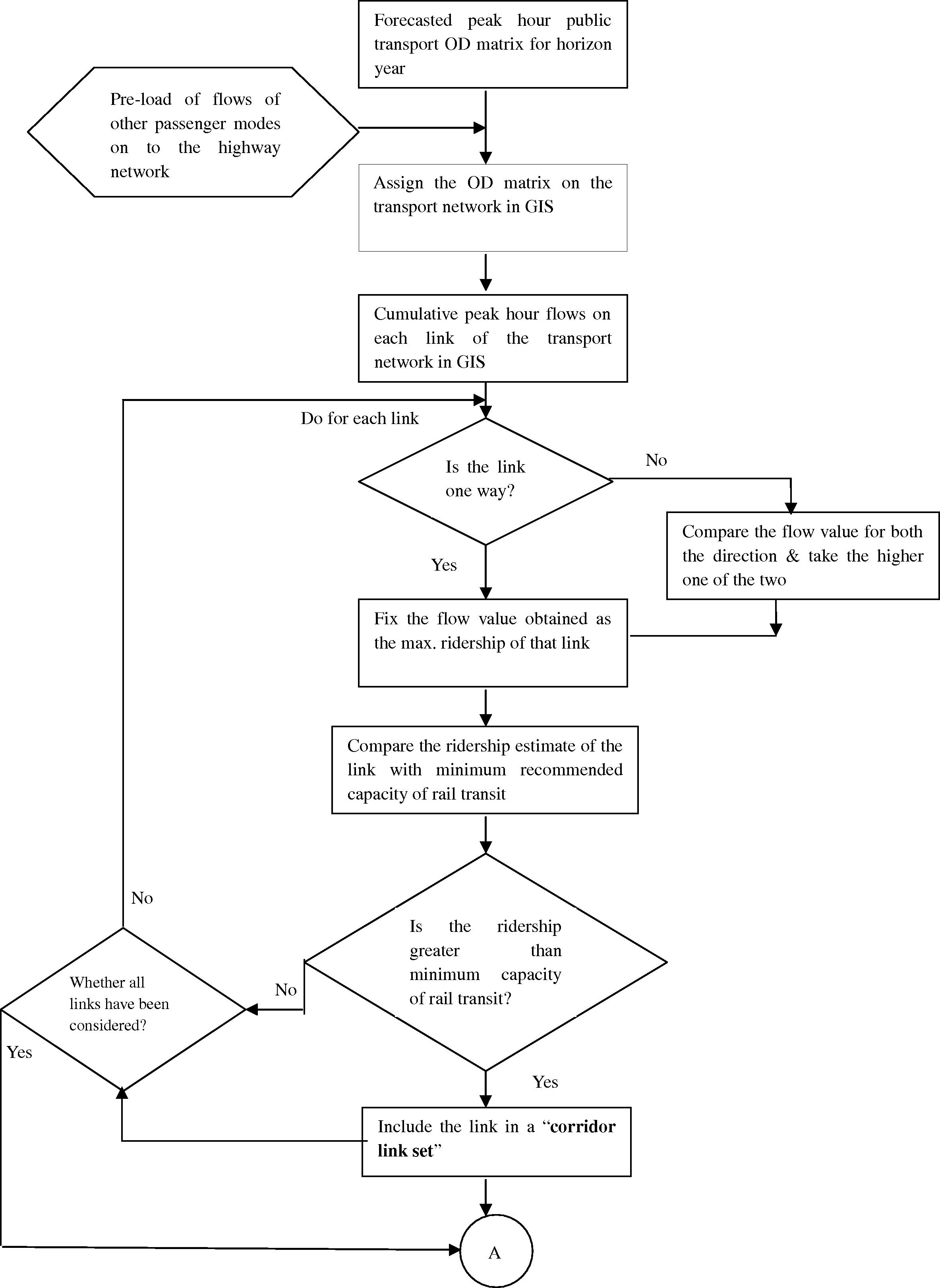
Solution approach.
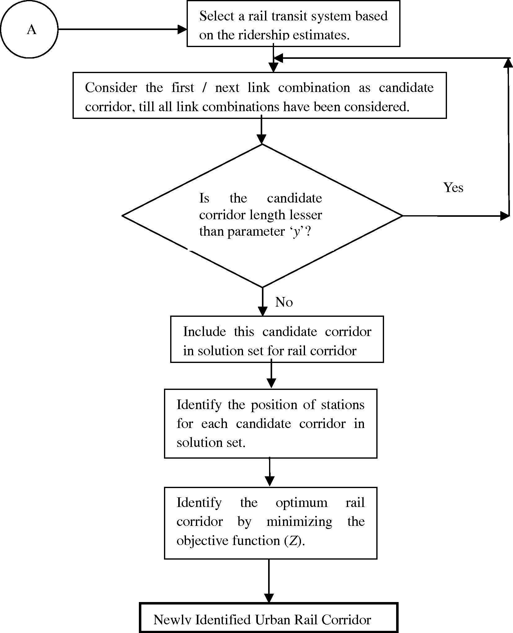
Solution approach.
The proposed model consists of three stages: public transport demand forecasting, creation of corridor link set, and optimization of rail corridor using GIS. The public transport demand forecasting is done primarily to get the required input data for the model, i.e., peak hour cumulative public transport O–D matrix for the planning year which is used later on for generation and optimization of rail corridor. It is performed using standard procedure and practice and no research contribution is claimed on this part of the work. It consists of four sub stages: base year O–D matrix generation, base year travel demand modeling, estimation of modal share for proposed rail transit mode, and forecasting of O–D person trip matrices.
3.3.1 Public transport demand forecasting
The base year O–D person trips matrices were generated from household interview survey data. In this stage, the model requires home interview survey, screen line, cordon line and network data. Base year travel demand modeling involves development of trip end and trip distribution models. Trip end models are developed only for intra-city trips made by residents of the study area, using stepwise multiple linear regression technique. All external trips are modeled by growth factor method. A doubly constrained gravity trip distribution model is calibrated to represent base year travel pattern for intra-city trips within the study area.
Now, it is expected that if an efficient and effective rail transit system is planned for any city, which is optimum from both user’s and operator’s point of view, there will be shift in mode share from all other passenger (OP) modes to proposed rail mode, which will help in maintaining a desired mode share between public transport (bus and rail) and other modes (making the city balanced and sustainable), and which is the ultimate goal of integrated mass transit planning. To obtain modal share of proposed rail transit mode, this shift from all OP modes to rail transit mode, is required to be found out. The shift can be estimated by conducting a detailed Stated Preference (SP) Survey, to model the choice of commuters between OP modes and proposed rail mode. Since this survey has to be conducted in absence of the network details of the proposed rail mode (which is essentially to be arrived at through the proposed model), the survey has to be carefully designed based on the target attributes of the integrated public transport system to be developed through the study. Mode wise binary logit models, which give probability of shift from each existing mode to proposed rail mode can be developed using preferences indicated by respondents. Here, it is assumed that all the commuters currently using bus mode will also be a part of mode share of integrated public transport system (rail and feeder bus system). This assumption holds reasonably well because after rerouting of bus system as feeder service to rail system the commuter will perform journey partly on feeder buses and partly on rail system. To check the reasonableness of the obtained mode share for integrated PT system, the same can be compared with desired modal share of public transport (if available) based on city population, size, and other attributes.
Finally, the daily O–D person trips matrix for the planning year is forecasted using trip end and trip distribution models developed for base year and also the mode share obtained from SP survey data. While forecasting the planning variables for trip end models the expected land use changes for the horizon year are taken into consideration. The daily matrix obtained is factored by average daily to peak hour ratio, in order to obtain peak hour O–D person trips matrix. This peak hour matrix is then factored by derived mode share of public transport to obtain the peak hour public transport matrix for horizon year. This matrix is used as an initial input in next stage for optimization of rail corridor using GIS.
3.3.2 Creation of corridor link set
By and large, the form and structure of Indian cities are not ideal (circular, semicircular or linear/grid), where the rail corridor could be simply aligned on corridors of heavy flow between residential zones and central business district. There is always some haphazard development of residential and work zones. This haphazard development leads to some level of discontinuity and randomness in the demand intensity on the city transport network which is observed in the form of a set of transport links having very heavy flow which may be beyond the capacity of street transit system to handle. Often these links indicate many continuous bands on the city transport network for small distances. These bands can be a part of the larger rail corridor which optimally connects many such bands. The set of these transport links having very heavy flow which may be beyond the capacity of street transit system to handle, is referred here as “corridor link set”.
To identify this corridor link set, the forecasted peak hour public transport O–D matrix for horizon year is assigned onto the base year transport network in GIS, using user equilibrium approach. This will give future public transport ridership pattern in terms of pphpd on every link of the transport network. Here, the base year bus transport network is not considered as it may not be optimum for the planning year and may create some bias toward finding an optimal solution. If a link is two-way then the flow value for both directions are compared for the higher one, which is fixed as the maximum peak hour ridership of that link. Flow value for a one-way link is used as it is. Further, if the maximum ridership estimate of a link is beyond the capacity of the street transit to handle then it is included in the corridor link set. Similar analysis is done for all the links, to arrive at the complete corridor link set.
3.3.3 Identification of rail corridor using GIS-based iterative algorithm
The corridor link set can provide many link-combinations for the formation of rail corridor. For instance, consider an example city network in Fig. 2. It shows a part of a city network joining central business district (CBD) and a residential belt. The corridor link set contains the following grouped links:
-
C-1-2-3
-
10-9-8-5-21-22
-
18-19-20
-
5-6-7
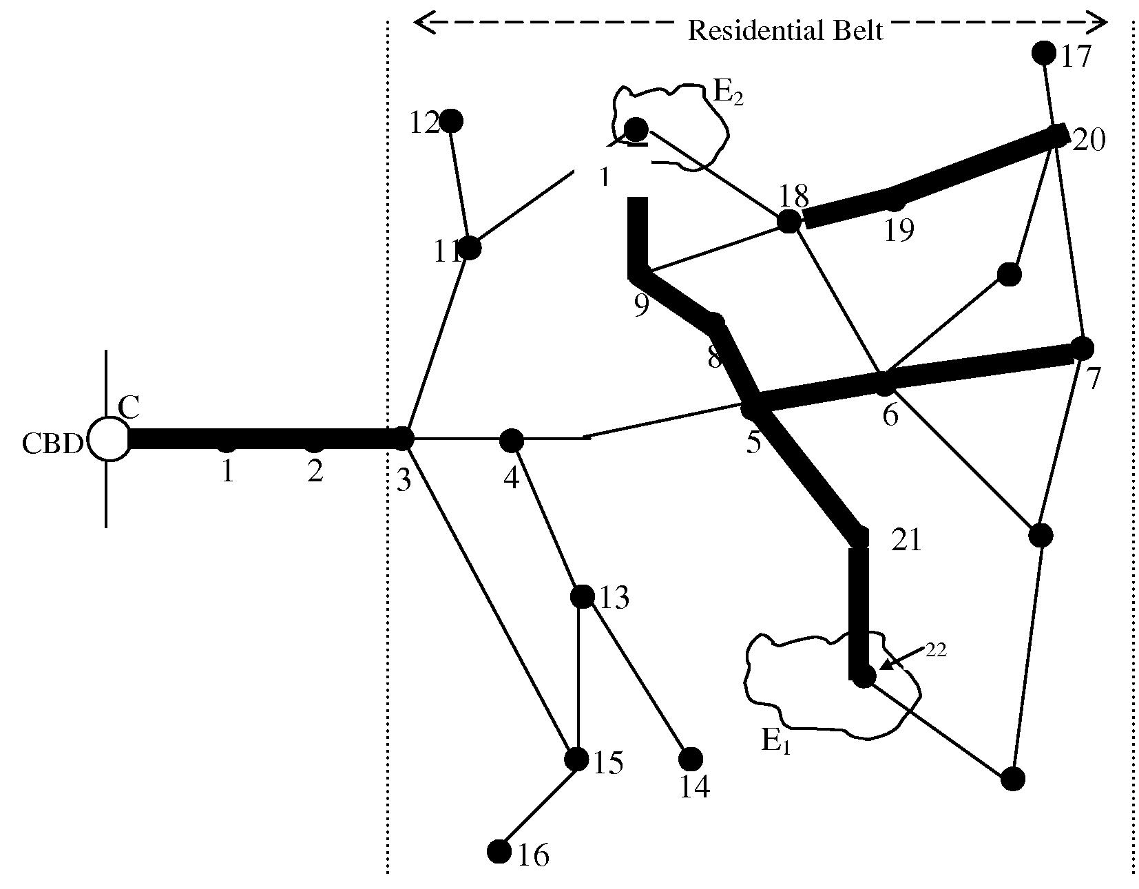
- Example City Network.
The proposed rail corridor can be aligned along various combinations of links. Some of these link-combinations for the example city are:
-
C-1-2-3⋯5-6-7
-
C-1-2-3⋯10-9-5-21-22
-
C-1-2-3⋯18-19-20
-
C-1-2-3⋯21-5-8-9-10
-
20-19-18⋯10-9-5-21-22, etc.
For an actual city, there may be several such link-combinations as potential candidates for the rail corridor. Considering the complexity of the model, lengthy procedure, and substantial data requirements; it will be computationally and time wise prohibitive to test the fitness of each candidate, some of which may be clearly impractical. One of the important aspects, to be examined here, is the minimum length of a rail corridor. The total length of a candidate rail corridor should be more than a pre-specified value of parameter y. This rule ensures that the proposed corridor should not be too small so as to be of no practical value for the user and also justifies the investments made by the operator (particularly for rolling stock, crew, and administrative staff, etc., which have not been taken into account explicitly in the model). The value of parameter y should be set such that the corridor covers the study area effectively and the access and egress time forms a smaller percentage of total O–D travel time of the user; otherwise the system will become unattractive to the user and will, therefore, affect the actual mode share and correspondingly the ridership and revenue generated from the new system after implementation. The value of y should be in correspondence with the values of various related parameters used earlier in the stated preference (SP) survey design for estimating the mode share of new rail system.
After arriving at the final set of candidate rail corridors, stations are identified using GIS for each candidate corridor based on the minimum and maximum inter-station spacing criteria and land use characteristics (Verma, 2010). The minimum and maximum inter-station spacing criteria is decided in such a way that the travel time of a commuter from his origin to final destination via the integrated network is as close as possible to its actual shortest path along the city transport network. In other words, the station spacing is decided so as to keep the ratio of travel time of commuter (between his origin and final destination) by transit to that by auto as close to one as possible. The other factors considered are the system characteristics of the recommended rail technology, different travel regimes of station-to-station train movement, and train stopping time at stations.
This finally gives candidate rail corridors consisting of combinations of closely spaced links having high demand, which cannot be handled by street transit; and station locations corresponding to each candidate corridor. The most suitable candidate among these is the one, which minimizes the objective function Z. The same is chosen as the optimum rail corridor for the city.
4 Proposed train scheduling model
Given the origin–destination (O–D) matrix for the transit trips (for design period) and the underlying train network (with the required attributes), the problem of train scheduling is to optimally allocate transit units among various available routes and obtain the optimal train fleet size. Considering the O–D flows to be given and fixed, the number of passengers using each path will still be a function of the transit allocation because of the proportionate frequency criterion being applied while assigning the demand to each route. Thus scheduling can be considered as an optimization problem. For the operation of a rail transit, the user and the operator which are the two agencies involved have conflicting objectives to be satisfied in a single objective function. User will be concerned with waiting time, level of service, least in-vehicle time, etc. Operator will be concerned with minimizing fleet size, vehicle operation cost, maximizing profit, etc.
According to the previous study by Verma and Dhingra (2006), the objective function was taken as minimization of operating cost of trains (operator cost) and waiting time of passengers (user cost) subject to load factor constraint and waiting time constraint. The in-vehicle time of the passenger (user cost) was not included in the objective function and the dwell time (which influences both the operator and user cost) was considered as a constant. The current study attempts to improve upon these limitations. Also, proportionate frequency criterion has been applied for assigning demand on the overlapping stations. The objective function can be mathematically represented as follows:
Minimize:
4.1 Objective function
The formulation in Eq. (8) is a combinatorial type optimization problem. The user cost component consists of minimizing the total waiting time, in-vehicle time of the commuters. The operator cost component consists of minimizing the total vehicle operating cost. Here, the user’s and operator’s objectives are conflicting in nature, for example, decrease in waiting time will result in increase in vehicle operating cost for the operator. Also, the in-vehicle travel time is a variable and is a function of dwell time. The dwell time is again a function of total boarding and alighting at any station, which in turn will depend on the frequency/headway chosen during each iteration.
4.2 Constraints
The meaning of each constraint is briefly described as follows:
Constraint g1 states that the load factor on any train route k should be less than the maximum allowable load factor Lmax for the train on that route.
Constraint g2 assures that the load factor on any train route k should be more than the minimum allowable load factor Lmin for the train on that route.
Constraint g3 assures that the waiting time incurred while traveling between station pair i, j along train route k should be less than the maximum allowable waiting time twt,max for commuter on that route.
Constraint g4 states that the waiting time incurred while traveling between station pair i, j along train route k should be more than the minimum allowable waiting time twt,min for the commuter on that route.
4.3 Solution approach
Since, the expected search space and train network is not very large, it is possible to work with total solution space and hence an exhaustive search algorithm (ESA), developed in MATLAB is used to minimize the objective function and obtain the optimum results. The number of trains to be run on each route and the total fleet size of trains can be obtained after getting the optimal frequency for each route from ESA. The following are the steps involved in the algorithm:
Step 1: Input data required comprises of, number of passengers boarding and alighting at each station within a fixed period, the train route details, the ridership estimate on each link of the train route, round trip time for each route, value of waiting time, travel time cost of passengers and train operating cost.
Step 2: Set the upper limit and lower limit of the variable headway.
Step 3: Start the loop and generate different set of headway for train routes, give the variable for minimum fitness function value, a very high initial value.
Step 4: Calculate the dwell time at each station.
Step 5: Calculate the objective function value for the given set of headway for the train routes.
Step 6: In case of violation, calculate the penalty for load factor and waiting time constraint and add it to objective function to obtain the unconstrained objective function value for the set of headway for train routes.
Step 7: Compare the fitness value with minimum fitness value obtained in previous iteration if it is less then assign the current fitness value to the minimum fitness value variable.
Step 8: Generate the next set of headway and go to Step 3.
Step 9: Iterate till all possible sets of route headways are processed for fitness value. Finally, report the global minimum fitness value and the corresponding solution details.
5 Case study
5.1 Study area details
The model is applied on Thane municipal corporation (TMC) area, a major urban center of Mumbai metropolitan region (MMR), India (Fig. 3). The population of Thane in base year 2001 is 1.26 million, it is expected to reach 3.04 million by the planning year 2031. The base year share of public transport is 34%.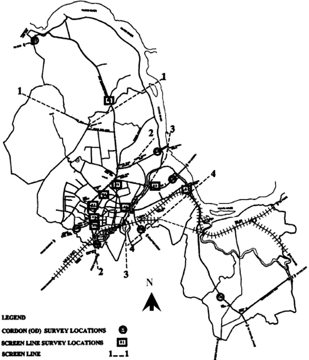
Map of the Study Area Thane.
5.2 Forecasting of public transport travel demand for study area
The base year O–D person trips matrices were generated from base year data. Also, trip end and trip distribution models were calibrated in TransCAD using the required base year data. The details and results of these stages can be referred in Verma and Dhingra (2003). The binary logit mode choice model was used to obtain percentage shift from existing modes to proposed rail mode in the horizon year (Verma, 2010). After obtaining the percentage shift, actual mode share of public transport in horizon year was calculated by adding actual shift from each existing mode to proposed rail mode and was obtained as 65%. This value of public transport share is reasonable if compared with desired PT share for Indian cities, as given in Table 1. The actual public transport share is used along with the daily to peak hour ratio of 8 to forecast horizon year peak hour public transport matrix using the models developed for base year (Verma and Dhingra, 2005). The matrix obtained thus forms a basic input for the identification of rail corridor.
City population (in millions)
Mass transport
Bicycle
Other modes
0.1–0.5
30–40
30–40
25–35
0.5–1.0
40–50
25–35
20–30
1.0–2.0
50–60
20–30
15–25
2.0–5.0
60–70
15–25
10–20
5.0+
70–85
15–20
10–15
5.3 Creation of corridor link set
To obtain the travel demand pattern for public transport (PT) modes, the forecasted peak hour public transport O–D matrix (obtained earlier) is assigned on base year transport network as per user equilibrium approach, to obtain ridership pattern in terms of pphpd on each link of network. Fig. 4 shows forecasted ridership pattern on study area map, as generated in TransCAD.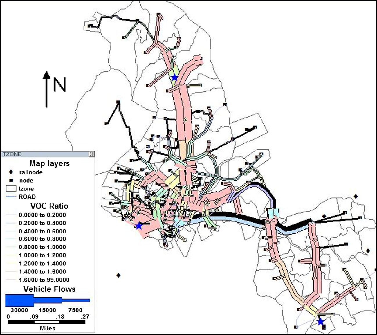
Forecasted ridership pattern on the transport network.
To obtain rail transit demand pattern and the corridor link set, the peak hour ridership obtained for each link (higher one out of the two directions in case of a two-way link to account for critical link flow) is compared with minimum recommended capacity of rail transit system, i.e., 12,000 pphpd [value referred from Verma and Dhingra (2001)]. All such links on the city transport network, which have got peak hour ridership more than minimum recommended capacity for rail transit were sorted and grouped together to form a corridor link set in GIS, the number of links included in this set were 37 in number, Fig. 5. These links emerge in almost continuous band except at few locations. This discontinuity is due to high diversion of ridership at some of the nodes. The maximum peak hour ridership in the network was found to be on link no. 85 as 34,369 pphpd. Hence, the most suitable system recommended for the operation on the newly identified corridor is light-rail transit (LRT) 1 running on right-of-way category B or C. Here, the capacity ranges were taken for different mass transit systems as: Street transit system = Up to 12,000 pphpd (Mini-bus, single decker standard bus, double-decker and articulated); LRT1(R/w category B or C) = 12,000–36,000 pphpd; LRT2(R/w category A) = 36,000–50,000 pphpd; RRT (Metro) = 50,000–69,000 pphpd; RGR (Regional Rail) = 59,000–89,000 pphpd. More detailed calculations of the above values can be found in Verma and Dhingra (2001).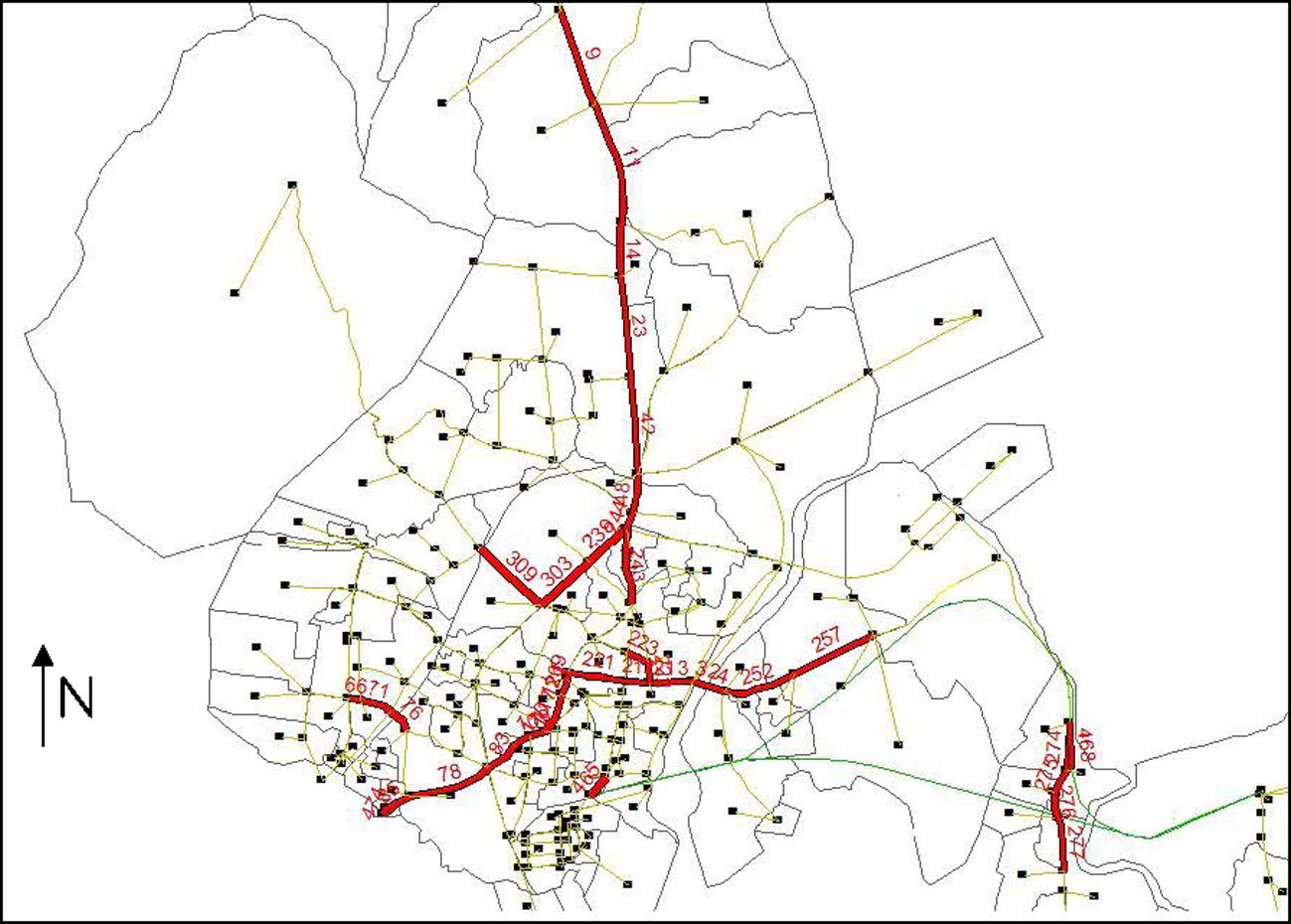
Corridor link set.
To carry out the initial screening of all possible link-combinations, the value of parameter y has to be carefully chosen such that the access time forms a smaller percentage of total O–D travel time of the user. For this, a sensitivity analysis was done to understand the change in weighted average accessibility distance with change in corridor length, as shown in Fig. 6. It can be seen from the figure that the accessibility distance becomes very high and increases sharply with decrease in corridor length beyond 7 km, accordingly, for the present study the value of parameters y has been taken as 7 km. Further, after applying the parameter y, a total of six candidate rail corridors were identified, and the objective function value (Z) was obtained for each one of them as per Eq. (1).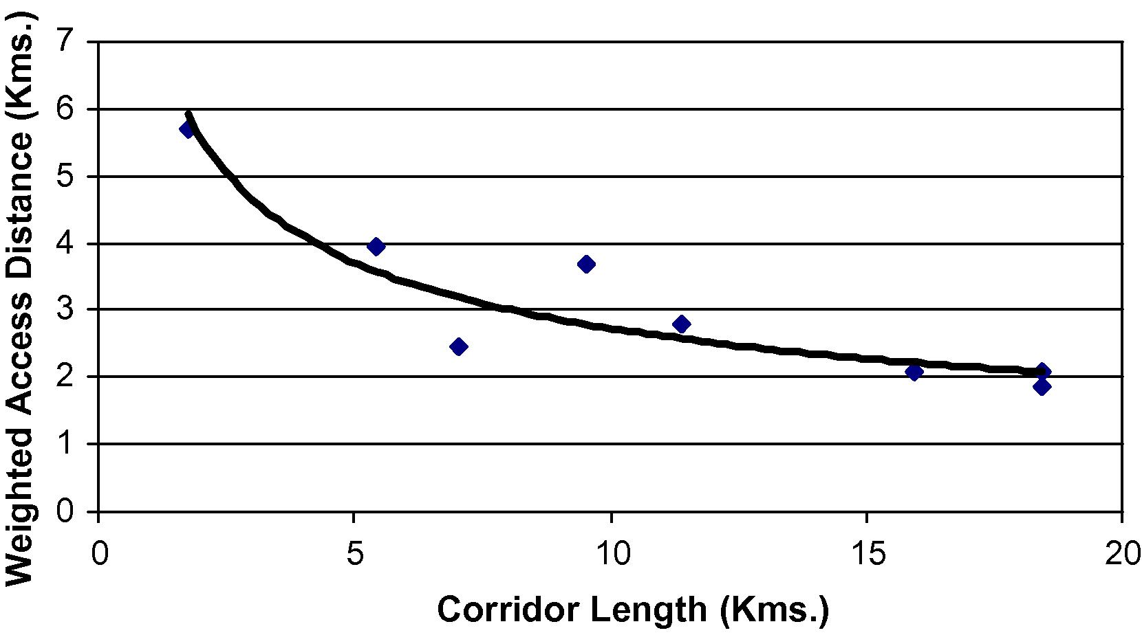
Variation in weighted average accessibility distance with corridor length.
5.4 Optimization of rail corridor using GIS
Firstly, the stations were identified on each of the candidate corridors based on the minimum and maximum inter-station spacing criteria (Verma, 2010). The nodes identified as possible locations of stations are; 8, 10, 12, 16, 25, 36, 43, 153, 157, 148, 70, 164, 165, 169, 170,182, 184, 186, 210 and 143. The six major corridors and their stations are shown in Figs. 7–12. The following sub-sections describe the cost calculations for deriving the objective function value.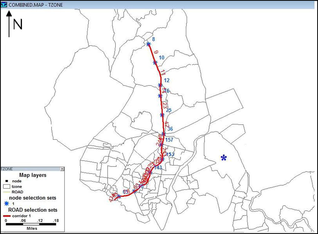
Corridor number 1.
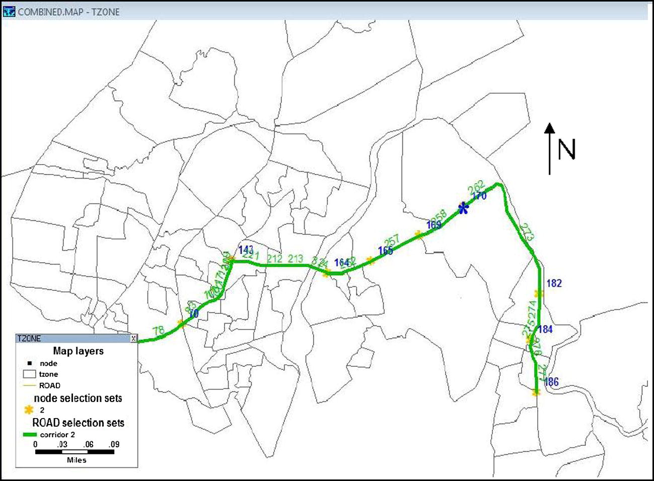
Corridor number 2.
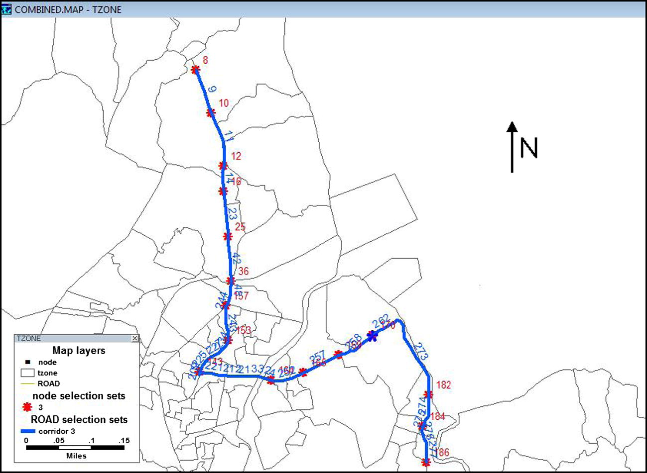
Corridor number 3.
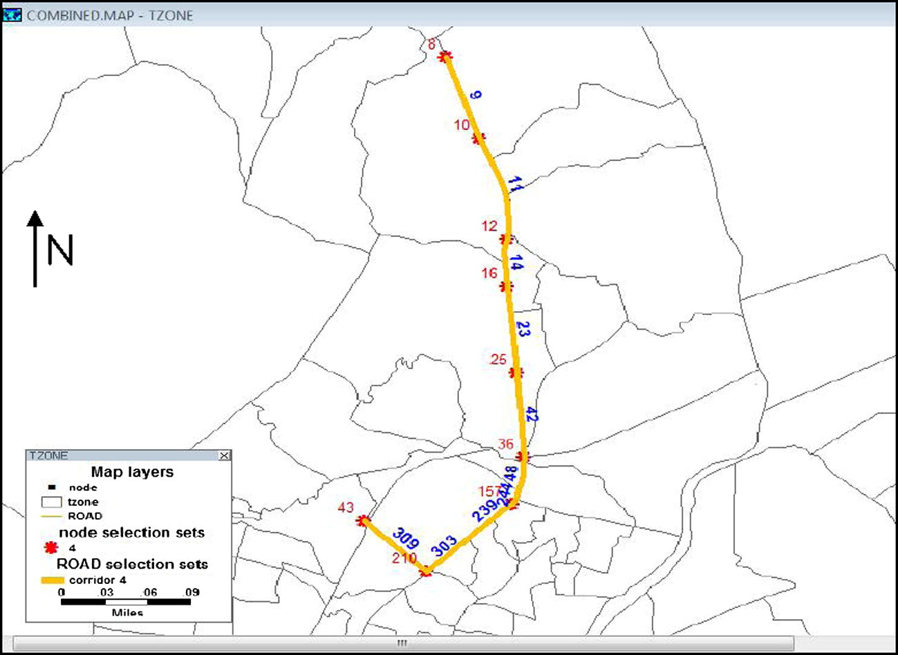
Corridor number 4.
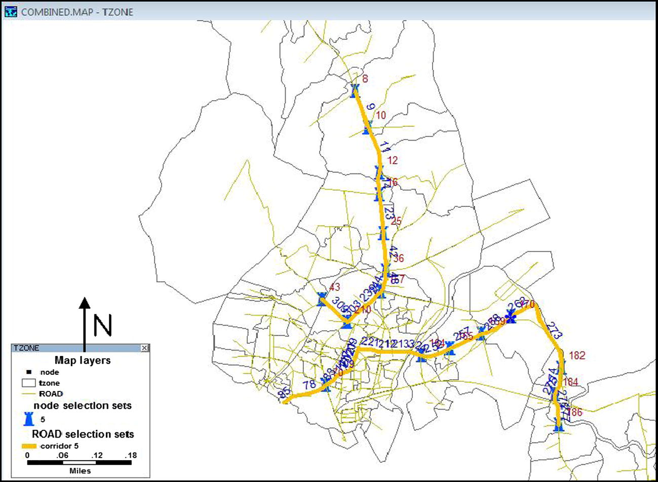
Corridor number 5.
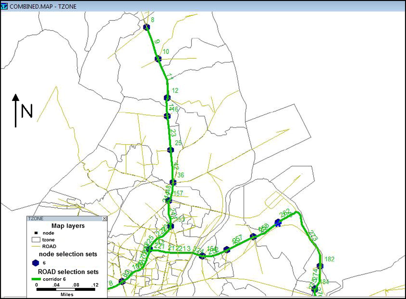
Corridor number 6.
5.4.1 Construction cost
Using Eq. (2), the construction cost is calculated for all the six corridors separately. The values of the required external parameters are: γl = Rs. 53,00,00,000/- per km of alignment obtained from CES (2001); ρ = Rs. 9.93% obtained from (CES, 2001); n = 30 years. The length of each candidate rail corridor along with the total construction cost is summarized in Table 2. Apparently, the construction cost increases with the corridor length and hence, corridor nos. 5 and 6 with maximum length of 18.45 km have the highest construction cost of Rs. 1,18,413/- per hour.
Corridor No.
Corridor length (km)
Weighted average distance of zone centroids from the stations (km)
Construction cost (Cc) in Rs. per hour
Operating cost (Oc) in Rs. per hour
User cost (Uc) in Rs. per hour
Total cost (Z) in Rs. per hour
1
9.54
3.7
61,228
20,623
3,098,680
3,180,531
2
11.41
2.8
73,230
25,693
2,407,285
2,506,208
3
15.95
2.1
102,368
54,326
1,924,691
2,081,385
4
7.04
2.45
45,183
11,869
2,061,425
2,118,478
5
18.45
1.86
118,413
63,351
1,766,852
1,948,616
6
18.45
2.08
118,413
63,353
1,978,209
2,159,975
5.4.2 Operating cost
Using Eq. (3), the operating cost is calculated for all the six corridors separately. The values of the required external parameters are: γoperating = Rs. 480/- per minute obtained from MMRDA (2000); Ro = 2 (in the absence of the availability of schedules, it is assumed constant for all candidate corridors); Tsj and Tj values are obtained from GIS data. The total operating cost for each corridor is summarized in Table 2. It can be seen that corridor no. 5, although having higher construction cost, has got the least operating cost of Rs. 63,351/- per hour.
5.4.3 User cost
Using Eq. (4), the user cost is calculated for all the six corridors separately. The important input for calculating the user cost is the estimate of the number of public transport passengers that are accessing/moving out from the individual stations by walking and by feeder mode. Here it is assumed that, within the feeder area of the station, all the public transport passengers whose origin is within 500 m radius from the station will access or egress by walk and rest will access or egress by feeder mode. Accordingly, simple overlay analysis in TransCAD was used to obtain these figures for each of the station of each candidate corridor. It is to be noted that these figures may be different between candidate corridor for the same station, as the feeder area of the station may change based on the layout of the candidate corridors. The values of the required external parameters are: γwalk = Rs. 0.15/- per minute per person, obtained from Verma (2010); γriding, γother = Rs. 0.5/- per person per minute, obtained from Verma (2010). Figs. 13a and b show the sensitivity of average riding time and walking time cost on the total objective function value. The figure shows that although the objective function value varies along with the average cost values however, the optimum solution remains the same. The total user cost for each corridor is summarized in Table 2. Further, the weighted average distance of zone centroids from the railway station is also calculated for each corridor (Table 2), which depicts the average accessibility of each candidate rail corridor. Implicitly, the corridor which is relatively away from the zones with larger production or attraction has higher average distance traveled by the user to the station, which eventually leads to higher user cost. Accordingly, corridor no. 1, which has the highest average distance of 3.7 km has the highest user cost; whereas corridor no. 5, which has the least average distance has also got the least user cost. After calculating all the costs for each of the six candidate corridors, the objective function value (Z) in terms of total cost is obtained for each corridor, as given in Table 2. From the table it can be seen that corridor no. 5 is optimum as it has the least cost among all the candidate corridors. Also, Table 3 presents flow characteristics of each corridor, which basically depicts the demand intensiveness of each corridor. It can be seen that the average flow on each of the corridor is above the minimum recommended capacity of rail transit system, i.e., 12,000 pphpd (xt). Further, coefficient of variation of link flows is the 2nd least for corridor no. 5, indicating the demand intensiveness of the corridor. Therefore, within the integrated framework, corridor no. 5 is recommended as the optimum rail corridor for Thane city.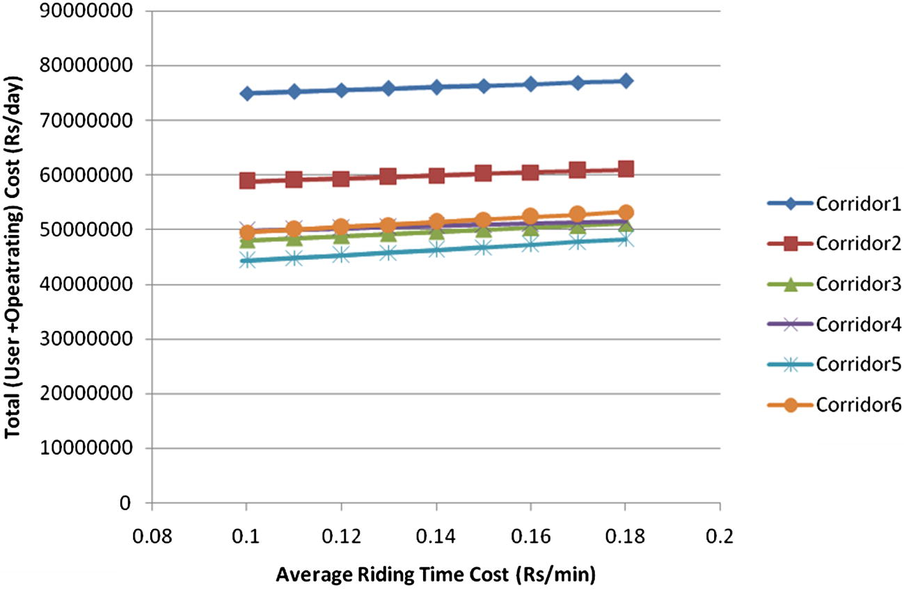
Average riding time cost vs. total objective function value.
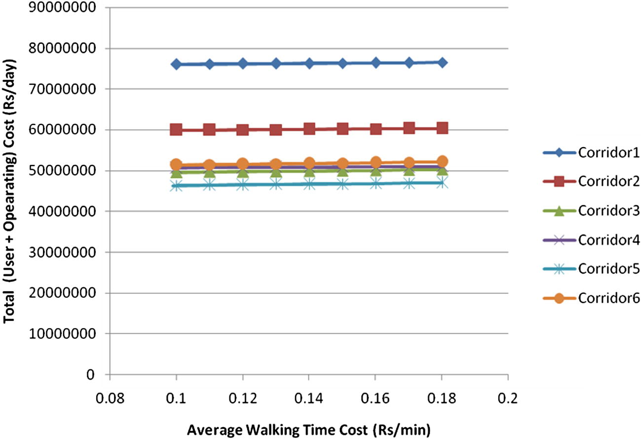
Average walking time cost vs. total objective function value.
Corridor No.
Average link flow
Standard deviation
Coefficient of variation
Minimum
Maximum
1
17,969
8050
45
4279
34,369
2
15,942
7823
49
1170
34,369
3
14,241
7227
51
1170
24,216
4
17,450
4585
26
12,896
27,260
5
16,428
6901
42
1169
34,369
6
16,330
7950
49
1169
34,369
5.5 Development of the train scheduling model
To avoid a additional transfer point and, therefore, to eliminate the discontinuity in the optimal corridor obtained, it was decided that the station number 43 and the corridor link 309 be omitted (as the link length is small and link flow is just above 12,000 pphpd level, which can be handled by feeder street transit system), and also, the disjointed links between stations 210 and 143 were connected and a continuous network was arrived at. Hence, the optimal corridor had the following 17 stations: 8, 10, 12, 16, 25, 36, 157, 210, 65, 70, 164, 165, 169, 170, 182, 184 and 186 (Fig. 14). Stations 8, 65 and 186 were taken as the terminal nodes and consequently schedules were obtained on the route between station 8 and 186 (Route 1) and 65 and 186 (Route 2). Table 4 shows the links between different station pairs and the distance between them and also the train ridership. The program for train scheduling model was coded and run in MATLAB.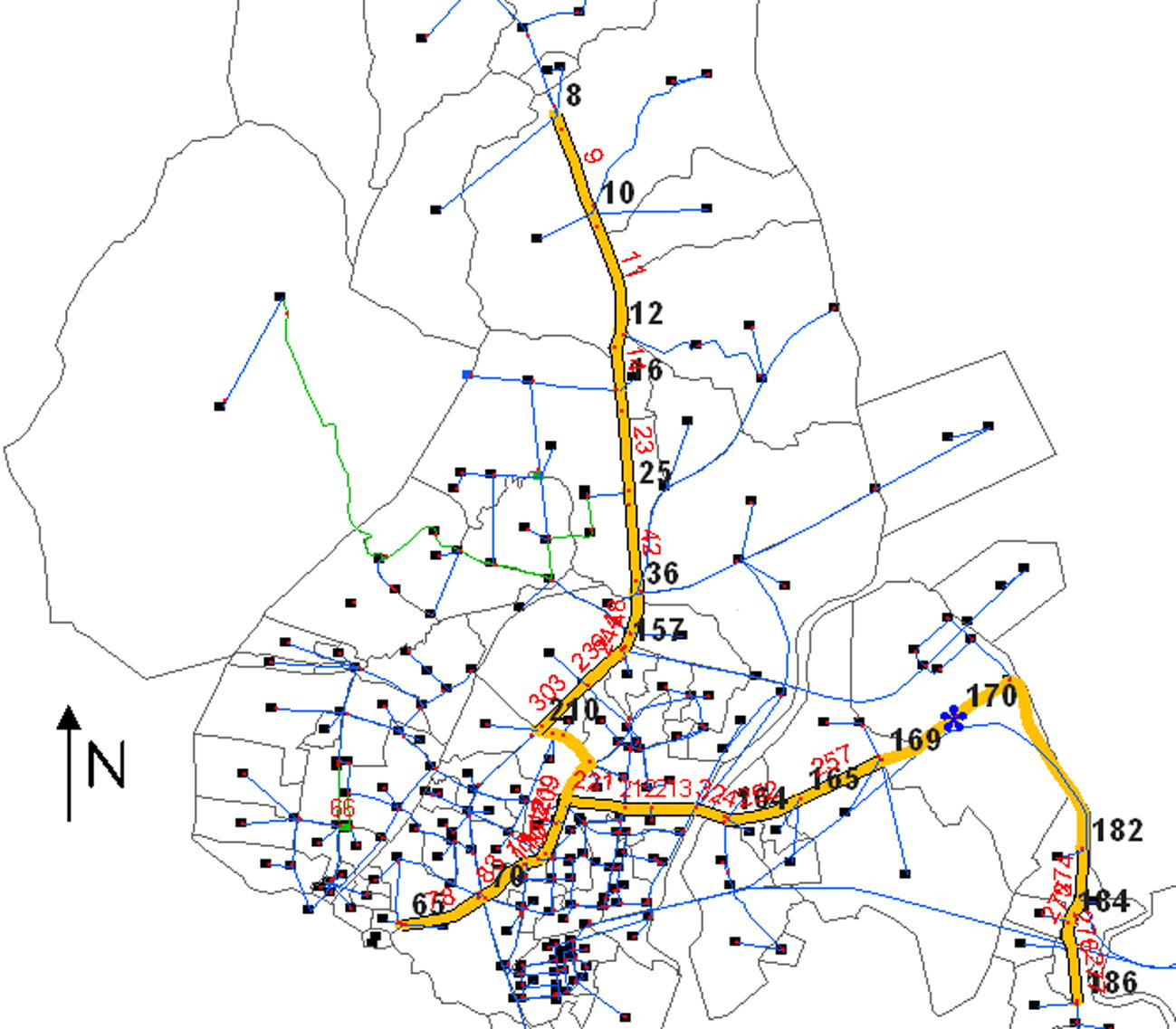
Modified optimal rail corridor in Thane city.
Route 1
Route 2
Station pair
Link ID
Length (Kms)
Ridership (pphpd)
Station pair
Link ID
Length (Kms)
Ridership (pphpd)
186–184
277
0.57
12,155
186–184
277
0.57
12,155
276
0.22
12,940
276
0.22
12,940
184–182
275
0.27
13,771
184–182
275
0.27
13,771
274
0.69
14,580
274
0.69
14,580
182–170
273
2.77
3522
182–170
273
2.77
3522
262
0.68
1169
262
0.68
1169
170–169
258
1.02
3621
170–169
258
1.02
3621
169–165
257
0.77
15,774
169–165
257
0.77
15,774
165–164
252
0.72
18,769
165–164
252
0.72
18,769
164–210
324
0.3
26,959
164–70
324
0.3
26,959
213
0.3
24,217
213
0.3
24,217
212
0.25
13,227
212
0.25
13,227
221
0.35
15,071
224
0.35
15,071
225
0.4
8002
209
0.1
20,074
228
0.4
7450
121
0.2
16,105
318
0.1
7587
117
0.3
16,176
304
0.2
8930
110
0.15
15,646
210–157
303
0.69
13,716
109
0.15
15,984
239
0.51
13,115
83
0.6
14,204
157–36
244
0.1
27,261
70–65
78
1
26,129
48
0.53
21,314
Total length 11.4 Kms
36–25
42
0.83
17,378
25–16
23
0.9
18,386
16–12
14
0.7
18,302
12–10
11
1.03
19,159
10–8
9
0.9
12,974
Total length 16.2 Kms
The train scheduling model is developed to obtain the optimal frequencies for rail operation on the newly identified rail routes (Fig. 14) and also to find the total number of trains required for each route and thus the total train fleet size required for the study area. The external parameters, which are required before running the ESA, are enumerated below.
-
Cost of waiting time = Rs. 0.15/min [adopted from MMPG (1997)]; cost of in-vehicle time = Rs. 0.12/min [adopted from MMPG (1997)]; train operating cost = Rs. 480/min [adopted from MMRDA (2000)]; lay over time = 5 min; Average train speed = 50 kmph; minimum allowable headway for LRT1 = 1 min [Verma and Dhingra, 2001]; seating capacity for LRT1 (for 2-vehicle train) = 130 [Verma and Dhingra, 2001]; minimum allowable load factor = 0.3; maximum allowable load factor = 1.0.
-
The penalty for load factor constraint g1 was taken as directly proportional to the load factor (penalty = obj * lf) when the pphpd > 36,000 or lf > 1 and inversely proportional (penalty = obj/lf) when the pphpd < 12,000 or lf < 0.3. This helps in appropriately accounting the penalty of load factor which is greater than 1 or less than a minimum value.
-
The minimum allowable waiting time for constraint g4 was taken as 0.5 min while g3 was suitably taken as 4 min. The penalty for waiting time constraint, i.e., g3, g4, was decided after number of trials and was taken as 0.5 times the objective function for both. The purpose of trials was to find the penalty value such that the objective function component and various constraints get equal weightage.
-
The range of decision variable (headway) was taken as 1–10 min.
Here, the minimum and maximum allowable load factor for the case study application is taken corresponding to the lower limit (12,000) and upper limit (36,000) in passengers per hour per direction (pphpd), respectively, of suitability range of light-rail system obtained from Verma and Dhingra (2001). This is done to maintain a minimum acceptable level of ridership in train from operator’s point of view and also to maintain the load factor in the train to be within the acceptable comfort level of the users in the case study area. With the input of these external parameters, the exhaustive search algorithm (ESA) was run for obtaining the optimal train frequencies for peak period and the fleet size. The output of the algorithm is as given below:
Headway for Route 1 is 4.4 min and for Route 2 is 10 min; Load Factor on Route 1 & Route 2 = 0.34 & 0.26, respectively; Round Trip Time for Route 1 & Route 2 = 69.6 & 55.1 min, respectively; Fleet Size for Route 1 & Route 2 = 16 & 6, respectively; Total Train Fleet Size = 22.
The sensitivity analysis of the minimum allowable load factor value reveals that with a decrease in its value, the optimum headway value also decreases. This is reasonable since a lower headway (or higher frequency) of trains leads to lesser passenger per trains and, therefore, lower load factor. Also, Fig. 15 shows the sensitivity of total objective function value with respect to variation in average waiting time cost. It was observed that although the objective function value increases with increase in the waiting time cost value, but the optimum solution does not change. Similar conclusion was made from the sensitivity of other cost parameters also. It can be seen from the results that the optimal headway required for the two routes in peak period came out to be 4.4 and 10 min, respectively. The frequency of the Route 1 as compared to the Route 2 is higher because of the higher demand intensity in the former. The first route passes through the denser region of Thane. To maintain this headway, the fleet size required for peak period is 22 trains. This is for the round trip time of 69.6 & 55.1 min for Route 1 and Route 2, respectively. Also, the load factor achieved for both the routes is close to the minimum allowable load factor, this ensures that there is adequate ridership in the train from operator’s point of view and at the same time the load factor does not reach toward the maximum allowable load factor corresponding to crush capacity of train, to increase the discomfort level of users.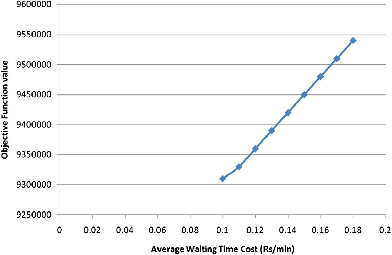
Average waiting time cost vs. total objective function value.
6 Conclusion
The major conclusions from study are as follows:
-
The proposed methodology addresses several shortcomings of previously developed methodology by Verma and Dhingra (2005) for rail corridor identification. The present approach is more exhaustive as it includes; construction cost, operating cost, riding cost, and access/egress cost.
-
The present work improves upon the previous work of Verma and Dhingra (2006) on train scheduling by developing a model that additionally incorporates in-vehicle time of the passenger (user cost) and also considers dwell time (which influences both the operator and user cost) as a variable, instead of constant, in the objective function. Thus the present model incorporates the decisive parameters more comprehensively than the previous approaches on train scheduling.
-
The corridor no. 5 is recommended as the most suitable corridor for the study area from user’s and operator’s point of view. It has the least objective function value, which includes the construction, operating and user costs. Corridor no. 5 also has the least weighted average distance of 1.86 km. from all the zone centroids to the identified stations on it. This shows that the corridor is most accessible and will be suitable for the daily commuters.
-
The train scheduling model is able to identify optimal schedules and fleet size for train operation, by optimizing the in-vehicle time, waiting time, and vehicle operating cost subject to constraints for waiting time, and load factor. For the study area, the optimal headway obtained for both the routes are within 10 min, hence, the average waiting time is not more than 5 min on any of the train routes.
The effect of change in land uses and change in O–D pattern due to provision of a new rail transit corridor has not been accounted for in the model. The availability of land for rail corridor has also not been directly accounted. Hence, these can also be treated as future scope of the work. To provide reasonably direct access to commuter from its origin to final destination, and also to achieve estimated ridership on newly identified rail corridor, a combined feeder route generation and schedule co-ordination model is developed, which along with rail corridor identification model and train scheduling model will satisfy the objectives of designing an optimum integrated urban mass transit system. The details of this model will be presented in subsequent papers.
Acknowledgments
The work presented in this paper is part of a sponsored project titled “Development of Simultaneous Approach for Integrated Mass Transit Planning”, funded by Department of Science and Technology (DST), Government of India, under the fast track scheme for young scientists (Project No. SR/FTP/ETA-25/2006). The authors would like to thank DST for this funding support.
References
- Consulting Engineering Services India Ltd. (CES), 2001. Proposed mass rapid transit for Thane city. Draft Final Report, MSRDC, Mumbai, India.
- Joint optimization of a rail transit line and its feeder bus system. Journal of Advanced Transportation. 1998;32(3):253-284.
- [Google Scholar]
- Strategic public transport planning in Baghdad. In: Heraty M., ed. Urban Transport in Developing Countries. London: PTRC Education Research Services Ltd.; 1991. p. :224-228.
- [Google Scholar]
- New technologies for transport route selection. Transportation Research. 2001;3(9):135-154.
- [Google Scholar]
- The determinants of light rail transit demand – an international cross-sectional comparison. Transportation Research. 1984;18(2):135-140.
- [Google Scholar]
- Optimal scheduling of trains on a single line track. Transportation Research. 1996;30B(2):147-161.
- [Google Scholar]
- Optimizing rail transit routes with genetic algorithms and geographic information system. Journal of Urban Planning and Development, ASCE. 2007;133(3):161-171.
- [Google Scholar]
- Tactical scheduling of rail operations: the SCAN I system. Transportation Science. 1991;25:46-64.
- [Google Scholar]
- Relationship between the number of stops and headway for a fixed-route transit system. Transportation Research A. 1985;19A(1):65-71.
- [Google Scholar]
- Optimal spacing of trains in freight railroads. Operations Research. 1991;39:82-99.
- [Google Scholar]
- Rail line length in a crosstown corridor with many-to-many demand. Journal of Advanced Transportation. 1996;30(1):95-114.
- [Google Scholar]
- MMPG, 1997. Techno-economic feasibility study of construction of Mumbai metro, Progress Report Submitted by MMPG to Govt. of Maharashtra, India.
- Mumbai Metropolitan Region Development Authority (MMRDA), 2000. Selection of a mass rapid transit system for Mumbai. Final Report for Greater Mumbai, The Andheri-Ghatkopar Corridor, Mumbai, India.
- Planning of integrated transit network for bus and LRT. Journal of Advanced Transportation. 1997;31(3):283-309.
- [Google Scholar]
- MOUD, 1998. Traffic and transportation policies and strategies in urban areas in India. Final Report. Ministry of Urban Development, Government of India, New Delhi.
- People for Modern Transit, 2001. Analysis of King county council transportation committee’s DMJM+Harris Tunnel Capacity Report, Washington, USA.
- On Some Problems in Railway Networks. Department of Operations Research, Case Western Reserve University; 1975.
- Timetables for a suburban rail transit system. Transportation Science. 1969;3:279-316.
- [Google Scholar]
- The minimum fleet size for a suburban railway system. Transportation Science. 1970;4:383-402.
- [Google Scholar]
- Srilakshmi, K. 1999. Optimum scheduling of trains in the context of suburban rail network, unpublished M-Tech thesis, Department of Civil Engineering, I.I.T., Bombay.
- Integrated Public Transportation System – Planning and Modelling. Mauritius: VDM Publishing House Ltd.; 2010.
- Suitability of alternative systems for urban mass transport for Indian cities. Trasporti Europei VII (18):4-15.
- [Google Scholar]
- Verma, A., Dhingra, S.L. 2003. Urban rail transport corridor identification. GIS Development, The Asian GIS Monthly, India, 7(5), pp. 39–42.
- Optimal urban rail transit corridor identification within integrated framework using geographical information systems. Journal of Urban Planning and Development, ASCE. 2005;131(2):98-111.
- [Google Scholar]
- Developing integrated schedules for urban rail and feeder bus operation. Journal of Urban Planning and Development, ASCE. 2006;132(3):138-146.
- [Google Scholar]


