An indirect measurement of the speed of light in a General Physics Laboratory

1 Introduction

Many properties of light have represented a major challenge to humanity for centuries. Aristoteles and Descartes believed that its speed was infinite until in the second half of the 17th century, the first measurements began to be made (Gonzalez Marhuenda, 2018). The speed of light in vacuum is a universal constant whose value in the International System of Units (SI) is $299792458m/s$, in the air its value is $299705543m/s$, and the speed does not depend on the reference system in which it is measured. It is represented by the letter $c$ which originates from the Latin term for speed, celeritas (Mantero Castañeda, 2016; NIST, 2014).

In 1638, Galileo Galilei attempted to measure c by using two lanterns with grilles which could be opened and closed as desired. On top of a hill near Pisa, an assistant placed a lantern and Galileo carried another one to another hill separated by one mile (Galilei, 1638). When Galileo opened his grille, the assistant, when the light was detected, in turn opened his grill and measuring the elapsed time, he could calculate the speed of light. The conclusion was that the speed of light was a very large value and it was not possible to obtain a specific value. In that period, there were no clocks that were capable of measuring with an accuracy of 10 µs. Likewise, the reaction time of a person is approximately 190 ms for a visual excitation and 160 ms for an auditory stimulus (Jensen, 2006).

In the second half of the 17th century, Roemer (Roemer, 1676; Vidal et al., 2010) was studying Io, which is the most internal Galilean moon of Jupiter. He discovered the delay in the appearance or concealment of Io in its orbit around Jupiter, when eclipses occurred. He observed that the time measured for 40 revolutions around Jupiter was significantly shorter when Jupiter and the Earth approached each other than when they moved away from each other; he consequently concluded that the observations were different due to the fact that light requires a finite time to reach the Earth from Jupiter. Roemer did not manage to calculate the speed of light, but with the data from that time, he would have obtained $2.15·{10}^{8}m/s$, with an error of 28%, which is an acceptable value when viewed with the perspective of 300 years later. With current data using the Roemer method, he would have obtained a value of $c=(2.98\pm 0.27)·{10}^{8}m/s$ (Mantero Castañeda, 2016).

In 1690, Huygens used the Roemer measurements and he observed that light takes 11 min to travel the distance which extends from the Sun to the Earth, which he estimated at $160·{10}^{6}km$ (Huygens, 1920). With this data, Huygens obtained $c=2.42·{10}^{8}m/s$. Now we know that light takes 8 min and 19 s to arrive from the Sun to the Earth. In 1782 when studying the aberrations of stars, Bradley obtained a value of $3.01·{10}^{8}m/s$ (Bradley, 1727; Mantero Castañeda, 2016). He estimated that the light originating from the Sun took 8 min and 12 s to reach the Earth.

In 1849, using a cogwheel and a mirror placed at distance of 8633 m (in the outskirts of Paris), Fizeau obtained a value of $c=3.13·{10}^{8}m/s$ (Fizeau, 1849). In 1853, Arago (Arago, 1853) concluded that the speed of light did not depend on the movement of the star which emitted it in relation to the Earth. This fact had very important consequences 5 decades later. In 1862, Foucault refined the measurement method by Fizeau and obtained a value of $2.98·{10}^{8}m/s$ (Léon Foucault, 1853). His method was so accurate that it only required that the light travel a distance of 20 m. In 1879, Morley measured the speed of light and obtained $c=3.00091·{10}^{8}m/s$. In 1926, he also obtained $c=2.9952·{10}^{8}m/s$ (Boyer, 1941).

In 1887, Michelson and Morley (Michelson and Morley, 1887) designed a meticulous experiment to measure the relative speed of light in relation to ether. At the end of the experiment, they concluded that the speed of light was constant, hence, ether does not exist. The experiment was a failure but at the same time, it was a successful experiment. A few years later among other evidence, this led to the appearance of Einstein’s Special Theory of Relativity.

In 1907, Rosa and Dorsey managed to obtain a value of $c=2.9988·{10}^{8}m/s$; in 1958, Froome was able to measure a value of $c=2.997925·{10}^{8}m/s$ using a microwave interferometer. In the 70 s decade, lasers were developed with a very large spectral stability and increasingly accurate cesium clocks, which greatly improved the measurements of $c$ until their absolute error reached $1m/s$ (Evenson et al., 1972).

At the present time, the speed of light is not a magnitude which is measured; it is a constant value within the current International System of Units. Hence since 1983 at the Conférence Générale des Poids et Mesures (CGPM) celebrated in Sèvres (Paris), the meter was defined as the length which light travels in a vacuum in a time interval equal to $\frac{1}{299792458}s$ which means, the speed of light is defined in an exact way as $c=299792458m/s$.

We have attempted to design an experiment in order to measure c in a General Physics Laboratory of the first University academic course without very complicated devices. Maxwell in his inaugural lesson, when he was appointed Professor at the University of Cambridge, stated the following: ‘… The simpler the materials of an illustrative experiment, and the more familiar they are to the student, the more thoroughly he is likely to acquire the idea which it is meant to illustrate. The educational value of such experiments is often inversely proportional to the complexity of the apparatus' (Maxwell, 2004). With this aim, we have designed the two experiments which we discuss below: an experimental calculation of the electric permittivity of free space and the experimental calculation of the magnetic permeability of free space using a smartphone. In addition to phone calls and messages, smartphones also allow us to perform multiple other activities such as measurements of movement, orientation, proximity to other objects, ambient light, linear or angular position, linear and rotational speed, acceleration, electric current and the three components of the magnetic field, among other physical quantities, because they are equipped with numerous Hall sensors.

Smartphones, due to their reasonable cost, size and various applications, which can be installed free of charge in them, are becoming powerful tools for data collection in physics laboratories for numerous practices related to mechanics (Monteiro et al., 2017; Monteiro and Marti, 2017; Pili and Violanda, 2018) and electromagnetism (Arribas et al., 2015; Arribas et al., 2020; Bonanno et al., 2017), among others. Besides, their effects on learning and their use in the classroom are being deeply analysed (Balaraman, 2015; Chuang, 2015; Goetz et al., 2017).

Finally, we shall briefly mention two articles which had the same objective. In the paper by Yuste et al. (Yuste et al., 1996) the electric permittivity of free space is obtained by a process that is more complicated than the one described herein: it studied the discharge of a capacitor, measuring the current intensity based on the voltage. The value which they obtain is ${\epsilon }_0=\left(8.6\pm 0.3\right)·{10}^{-12}F/m$. For the measurement of the magnetic permeability free space, an alternating current is used which supplies power to a coil of 200 turns, which generates an induced electromotive force in the centre of another smaller coil with 500 circular turns. Varying the effective value of the alternating current, they calculate the value of the magnetic permeability of free space. The value which they obtain is ${\mu }_0=\left(1.28\pm 0.04\right)·{10}^{-6}N{A}^{-2}$. They subsequently obtain the following value for the speed of light, with two significant figures, $c=\left(3.0\pm 0.1\right)·{10}^{8}m/s$, although they do not explain how the obtained the absolute error value.

In the article by Gimeno et al. (Gimeno et al., 2000), they measure the resonance frequency of a RLC circuit based on the distance between the capacitor plates. The particularity of this method is that they calculate the product of both magnitudes ${\epsilon }_0·{\mu }_0$ without measuring them separately. From there, they calculate the value in an indirect way for the speed of light which is $c=\left(3.00\pm 0.07\right)·{10}^{8}m/s$, although they also do not explain how they obtained the absolute value of the speed of light. The value of c which they obtain has three significant figures.

2 Experimental calculation of the electric permittivity of free space

2.1

2.1 Methodology

We consider a circular and parallel-plate capacitor of area A, separated at a distance d that is very small in comparison with its dimensions, as shown in the experimental set-up of Fig. 1.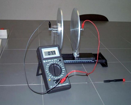

Close

Fig. 1

Measurement of the capacitance of a circular and parallel-plate capacitor using a capacitance meter.

Export to PPT

The capacitance of this capacitor is provided by

(1)

$$C={\epsilon }_0\frac{A}{d}$$where ${\epsilon }_0$ is the electric permittivity of free space. For practical effects, the vacuum and air are equivalent, above all for the accuracy range which we consider.

The capacitor which we use has circular plates of radius R, although we shall use the diameter D, which is much easier for the students to measure. The value of the diameter with its absolute error is as follows: D = 0.2600 ± 0.0010 m. Hence, the area of each plate is

(2)

$$A=\pi R^2=\frac{1}{4}\pi D^2$$

and the capacitance is shown below

(3)

$$C=\frac{{\epsilon }_0\pi D^2}{4}·\frac{1}{d}$$where it is clearly seen that the variables C and d are inversely proportional. In order to obtain the Eq. (1) this means that the electrical field inside the capacitor is uniform and perpendicular to the two plates. In order that the finite size of the capacitor does not affect the measurements, it was necessary to make the exact measurement in the centre of the capacitor, as distant as possible from the edges; we can then consider that the electric field is practically uniform. This detail was already resolved with the current capacitors when making the connections in the installed sites. Special care must also be taken so that both plates are parallel; this detail is crucial. If this is not the case, it would be necessary to rectify it.

Another important detail is the one that appears printed in the own capacitance meter. Before making each measurement, the capacitor must be discharged. The battery that has the capacitance meter in its interior transfers a small charge to the plates of the capacitor. This charge is necessary to be able to measure the capacitance of the capacitor, but it must be removed to start the next measurement correctly. That's why it is necessary to touch both plates at the same time to discharge them.

The capacitance is measured by a digital capacitance meter, as shown in Fig. 1. We use a 200 pF scale background. To ensure the correct measurements, it is necessary to adjust the zero setting of the capacitance meter with the two cables connected. Although slightly, the cables can have an influence on the total capacitance. We make this zero adjustment before each measurement. This process can may seem a little tedious, but it is absolutely necessary if we want to obtain an acceptable precision. The exact value of ${\epsilon }_0$, Eq. (5), has more than 10 significant figures. We obtain three significant figures (as we shall see below). This value in SI is

(4)

$${\epsilon }_0=8.854187817\cdots ·{10}^{-12}F/m$$

2.2

2.2 Experimental results

We measure the capacitance of the parallel plate capacitor based on the separation between its plates. Fig. 2 shows the experimental data obtained, as well as the corresponding linear regression and squared correlation coefficient.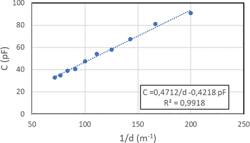

Close

Fig. 2

Graphic diagram of the experimental values of the capacitance of the capacitor (measured in pF) versus the inverse separation between the plates (measured in m⁻¹) and the straight line of the least squares adjustment. It also shows the equation of the straight line and the value of the squared correlation coefficient.

Export to PPT

Below, we make a least squares adjustment, obtaining in the SI the value of the slope, m, and the y-intercept, b, with their respective absolute errors, as well as the correlation coefficient:

(5)

$$m=\left(0.471\pm 0.015\right)·{10}^{-12}F·m$$

(6)

$$b=\left(-0.4\pm 1.9\right)·{10}^{-12}F$$

(7)

$$r=0.9959$$

Once the slope was known, we were able to obtain the electric permittivity of free space

(8)

$$m=\frac{{\epsilon }_0\pi D^2}{4}\Rightarrow {\epsilon }_0=\frac{4m}{\pi D^2}$$

by substituting we obtain

(9)

$${\epsilon }_0=8.8742·{10}^{-12}F/m$$

In Eq. (9) we see that ${\epsilon }_0=f(m,D)$ hence its absolute error is

(10)

$${\epsilon }_a\left({\epsilon }_0\right)=\sqrt{{\left[\frac{\partial {\epsilon }_0}{\partial m}{\epsilon }_a\left(m\right)\right]}^2+{\left[\frac{\partial {\epsilon }_0}{\partial D}{\epsilon }_a\left(D\right)\right]}^2}=0.29·{10}^{-12}F/m$$

with its relative error ${\epsilon }_r\left({\epsilon }_0\right)=3\%$.

Hence, the value obtained for the electric permittivity of free space, with its correct significant figures and its absolute error is

(11)

$${\epsilon }_0=\left(8.87\pm 0.29\right)·{10}^{-12}F/m$$

Evidently, the exact value for ${\epsilon }_0$ is within the error interval. We obtained three significant figures and a small relative error.

3 Experimental calculation of the magnetic permeability of free space

3.1

3.1 Methodology

Now we use the solenoid of length L, radius R and a number of turns N.

(12)

$$L=0.4000\pm 0.0010m$$

(13)

$$R=0.0600\pm 0.0005m$$

(14)

$$N=120$$

In Fig. 3, we can see a photo of the experimental set-up used. By means of a variable dc voltage generator, we make the current I pass through the solenoid which we will measure with a digital ammeter.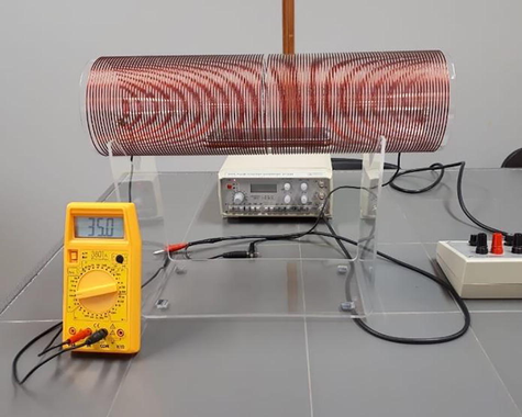

Close

Fig. 3

Experimental set-up to determine the magnetic permeability of free space, we can see a Smartphone inside the solenoid (acting as a Tesla meter, also called magnetometer), a variable dc voltage generator and a digital ammeter.

Export to PPT

We will measure the magnetic field inside the solenoid by inserting a Smartphone in it. We will use the magnetic field sensor of the Smartphone, in which we will have previously installed the app: ‘Magnetometer’ for iOS or ‘Physics Toolbox’ for Android (Arribas et al., 2015). This option of using a tool which almost all the students carry in their pockets permits a greater predisposition towards the experiment.

To reduce the contribution of the Earth’s magnetic field, we will place the solenoid in an East-West direction and with the corresponding app, we will measure the y-component of the magnetic field vector, see Fig. 4.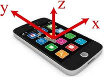

Close

Fig. 4

Orientation of the axis in a Smartphone. The measurements are made in the direction of the 'y' axis which must be perpendicular to the North-South axis.

Export to PPT

As a precaution, in case there are other residual fields in addition to the Earth’s magnetic field, we will have previously measured the initial value of $B_y$, which we will call $B_{y_0}$, when current does not pass through the solenoid, which is equivalent to the zero adjustment which we carried out in the previous section (Arribas et al., 2015).

The magnetic field of a finite solenoid in its centre is provided by the following expression

(15)

$$B_y=\frac{{\mu }_{0}NI}{2}\frac{1}{\sqrt{R^2+{\left(\frac{L}{2}\right)}^2}}$$

In the following, we are going to use an approximation to this expression, since L is quite higher than R

(16)

$$B_y={\mu }_0\frac{N}{L}I$$

In the SI, the numeric value of the magnetic permeability of free space is an exact value

(17)

$${\mu }_0=4\pi ·{10}^{-7}\frac{T·m}{A}=1.2566·10^{-6}\frac{T·m}{A}$$

3.2

3.2 Experimental results

Fig. 5 shows the experimental data obtained from the magnetic field inside the solenoid versus the intensity which passes through it, its corresponding linear regression and the squared correlation coefficient.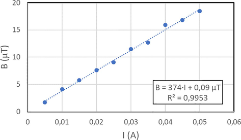

Close

Fig. 5

Experimental measurements of the magnetic field (measured in µT) inside the solenoid versus the current which passes through it (measured in A) and the straight line of a least squares adjustment. It also shows the equation of the straight line and the value of the squared correlation coefficient.

Export to PPT

By means of a least squares adjustment, we obtain in SI

(18)

$$m=\left(374\pm 9\right)·{10}^{-6}T/A$$

(19)

$$b=\left(0.09\pm 0.28\right)·{10}^{-6}T$$

(20)

$$r=0.9976$$

From Eq. (17) we see that the slope corresponds with

(21)

$$m=\frac{{\mu }_{0}N}{L}\Rightarrow {\mu }_0=\frac{\mathit{mL}}{N}=1.25·{10}^{-6}N{A}^{-2}$$

where we see that ${\mu }_0=f(m,L)$ hence its absolute error is

(22)

$${\epsilon }_a\left({\mu }_0\right)=\sqrt{{\left[\frac{\partial {\mu }_0}{\partial m}{\epsilon }_a\left(m\right)\right]}^2+{\left[\frac{\partial {\mu }_0}{\partial L}{\epsilon }_a\left(L\right)\right]}^2}=0.03·{10}^{-6}N/A^2$$

And its relative error is ${\epsilon }_r\left({\mu }_0\right)=2.4\%$.

Thus, the value obtained for the magnetic permeability of free space, with its correct significant figures and its absolute error is

(23)

$${\mu }_0=\left(1.25\pm 0.03\right)·{10}^{-6}N{A}^{-2}$$

The exact value of ${\mu }_0$ is within the error interval.

4 Indirect measurement of the speed of light

With the experimental set-ups explained in the above sections, we were able to obtain an indirect measurement of the electric permittivity and the magnetic permeability of free space:

With this data, we can perform the indirect calculation of the speed of light

Using the mean square error, we can calculate the relative error of the speed of light

Once the relative error is known, we can obtain the absolute error

Hence, the experimental result with the correct significant figures which we obtain for the speed of light in the air is

where the exact value of c, 2.99792458·10⁸ m/s is within the error interval. Working with amounts that have three significant figures, it is expected that the result will also have three significant figures.

5 Conclusions

With two measurements in the laboratory of a General Physics course, which means without large devices or excessive complications, we have obtained the value of two physics magnitudes, one with a relative error of 3% and the other of 2.4%. The final measurement of the speed of light has a relative error of 1.9%.

We have mentioned that it would be necessary to balance the two devices at the start of the measurements. In reality, the balance of the capacitance meter and the initial value of $B_y$ do not affect the slopes, they exclusively affect those y-intercept, however it is not necessary for us to consider them in our calculation.

These two practice sessions are done by our students from the first course (in the different degrees in which we teach classes). They are practice sessions in which the students handle the devices, perform the measurements and subsequently make several adjustments and mathematical calculations. The measurement of the speed of light, a well-known magnitude assimilated since very early ages, awakens an additional curiosity in the students’ desire to learn. We are convinced that this is important so that the students’ learning is meaningful.

In order for the laboratory to be efficient for learning, it must obtain the magnitude value with its corresponding absolute error and correct units. In addition, the real value of the magnitude (if it is known) must be within the error interval. If this does not occur, we should at least know which agents are interfering in the measurements so that the learning is constructive.

6 Discussion

In this section, we will discuss what happens if we use Eq. (16) instead of Eq. (17). The solenoid utilized has a relationship between its dimensions

Eq. (17) would be a very good approximation when this quotient, Eq. (31), was ≤ 0.1. For this reason, we will now use Eq. (15) to obtain the value of ${\mu }_0$. The new obtained value is 4% higher than the previous one, Eq. (24),

the exact value of this magnitude being slightly outside the error interval.

Re-calculating the speed of light we obtain a slightly lower result than the value obtained in Eq. (30), specifically the 2%

The exact value of c is within the error range. This new value is compatible with the one obtained previously.

References

- Measurement of the magnetic field of small magnets with a smartphone: a very economical laboratory practice for introductory physics courses. Eur. J. Phys.. 2015;36:065002
- [CrossRef] [Google Scholar]
- Measuring the magnetic field created by a linear quadrupole. Phys. Teach.. 2020;58:182.
- Physiotherapy Students’ Perception on Learning through Smartphone: A Pilot Study Physiother. Occup. Ther. J.. 2015;8:53-61.
- [Google Scholar]
- An innovative experimental sequence on electromagnetic induction and eddy currents based on video analysis and cheap data acquisition Eur. J. Phys.. 2017;38:065203
- Bradley, J., 1727. A letter from the Reverend Mr. James Bradley Savilian Professor of Astronomy at Oxford, and F. R. S. to Dr. Edmond Halley Astronom. Reg. &c. giving an account of a new discovered motion of the fix’d stars. Philosophical Transactions of the Royal Society of London 35, 637–661. https://doi.org/10.1098/rstl.1727.0064
- SSCLS: A Smartphone-Supported Collaborative Learning System Telemat. Inform.. 2015;32:463-474.
- Speed of Light from Direct Frequency and Wavelength Measurements of the Methane-Stabilized Laser. Physical Review Letters. 1972;29:1346.
- Galilei, G., 1638. Discorsi e dimostrazioni matematiche intorno a due nuove scienze [Document]. https://portalegalileo.museogalileo.it/igjr.asp?c=36308 (accessed 3.28.19).
- Determinación indirecta de la velocidad de la luz en el vacío mediante un circuito resonante. Revista Española de Física. 2000;14:41-44.
- Users of the main smartphone operating systems (iOS, Android) differ only little in personality. Plos One. 2017;12:e0176921
- La naturaleza de la luz: Breve historia bibliográfica (1st ed.). Valencia: ADAMA; 2018.
- Huygens, C., 1920. Traité de la lumière / par Christian Huyghens. gallica.bnf.fr. https://gallica.bnf.fr/ark:/12148/bpt6k5659616j
- Clocking the mind: mental chronometry and individual differences (1st ed.). Elsevier, Amsterdam: Boston; London. Library of Congress; 2006.
- Mantero Castañeda, E.A., 2016. Medición de la velocidad de la luz. Rehaciendo el Experimento de Römer. (Tesis de Fin de Grado). Universidad de la Laguna. https://riull.ull.es/xmlui/bitstream/handle/915/3052/Medicion%20de%20la%20Velocidad%20de%20la%20Luz.pdf?sequence=1
- Maxwell, J.C., 2004. Five of Maxwell’s Papers, Project Gutenberg eBook [Document]. URL http://www.gutenberg.org/ebooks/4908 (accessed 5.4.19).
- On the Relative Motion of the Earth and the Luminiferous Ether. Am. J. Sci.. 1887;34:333-345.
- Using smartphone pressure sensors to measure vertical velocities of elevators, stairways, and drones. Phys. Educ.. 2017;52:015010
- Magnetic field “flyby” measurement using a smartphone’s magnetometer and accelerometer simultaneously. Phys. Teach.. 2017;55:580-581.
- NIST, 2014. Fundamental Physical Constants from NIST - Background information [Document]. Constants, Units, & Uncertainty. https://physics.nist.gov/cuu/Constants/background.html (accessed 3.22.19).
- Measuring average angular velocity with a smartphone magnetic field sensor. Phys. Teach.. 2018;56:115-116.
- Démonstration touchant le mouvement de la lumière trouvé par M. Roemer de l’Académie des science. J. des Sçavans du lundi 1676.:276-279.
- Vidal, I.M., Monferrer, S.J., Molina C. de la, 2010. Emulando a Römer: medida de la velocidad de la luz cronometrando los eclipses Io Revista Española de Física 24 2010 48 51.
- Dos experimentos sencillos para la determinación de la permitividad eléctrica y de la permeabilidad magnética del vacío. Revista Española de Física. 1996;10:41-45.