An algorithm for outlier detection in a time series model using backpropagation neural network

1 Introduction

The detection of outliers or unusual data structures is one of the important tasks in the statistical analysis of time series data as outliers may have a substantial influence on the outcome of an analysis. Appropriate definition of an outlier usually depends on the assumptions about the structure of data and the applied detection method. Hawkins (1980) defined the outlier as an observation that deviates so much from other observations as to arouse suspicion that it was generated by a different mechanism. Barnett and Lewis (1994) indicated that an outlying observation, or outlier, is one that appears to deviate markedly from other members of the sample in which it occurs. Similarly, Johnson (1992) viewed that, an outlier is an observation in a data set which appears to be inconsistent with the remainder of that set of data. There are many definitions of outlier proposed in the literature of time series. Outlier observations in some situations are also referred as anomalies, discordant observations, or contaminants Carreno et al. (2019).

The presence of outliers in a time series has a significant effect on the results of standard procedures of analysis. The consequences may lead to improper model specification, faulty parameter estimation and substandard forecasting. A crucial point here is that any outlier detection technique can at most detect a set of data points having different behavior than the rest of the data and hence, it can be termed as a probable set of outliers. However, it is up an analyst to take various itineraries to come up with a final decision to justify these detected points as outliers. It is probable that a point detected as an outlier has some real facts behind it, e.g., the price of a stock just after the date of stock split with split ratio of 2-for-1 or 3-for-1, which means a stockholder gets two or three shares, respectively, for every share held. In a reverse stock split, a company divides the number of shares that stockholders own, raising the market price accordingly. In such a scenario, most of the outlier detection algorithms will detect the prices after the date of stock split as outliers. The impact of outliers on parameter estimation has been studied by Pena (1990), Fox (1972). Deutsch et al. (1990) explored the effects of a single outlier on autoregressive moving-average (ARMA) identification. In their study, Barreyre et al. (2019) used statistical outlier detection methods to detect anomaly in space telemetries. The suggested methods addressed the issue of outlier limited to the nature and number of outliers. Moreover, the some of the method of parameter estimation is based on maximum likelihood estimation or on the least square approach.

Outliers in a time series are usually generated by dynamic intervention models at unknown points of time. A common practice to deal with the outliers in a time series is to identify the locations of outliers and then to use intervention models to analyze the outlier effects. This is an iterative method that requires iterations between outlier detection and estimation of model parameters. Tsay (1988) discussed the significance of outliers in level shift and its dynamics that leads to change in variance of the series. In their findings, Chang et al. (1988) introduced two types of outliers, namely additive outliers (AO) and innovative outliers (IO). However, Chen and Liu (1993) later introduced two more types of outilers in time series such as temporary change (TC), and level shift (LS), addressing their effect in modeling and estimating the parameters of time series. They further demonstrated that the sensitivity of the forecast intervals are mainly due to AO and discussed the issue of forecasting when outliers occur near, or at the forecast origin. The consequence of additive outliers on forecasts was addressed by Ledolter (1989) in the case of ARMA model. In their study, Battaglia and Orfei (2005) discussed the problem of identifying the location of outliers and estimation of the amplitude in nonlinear time series. An alternative semi-parametric estimator for the fractional differencing parameter in the autoregressive fractionally integrated moving average (ARFIMA) model was introduced by Molinaresa et al. (2009) which is robust against additive outliers. In their study, Leduca et al. (2011) considered the implementation of auto-covariance function that is robust to the additive outliers. Loperfido (2020) discussed a method based on achieving maximal kurtosis for outlier detection in multivariate and univariate time series models. However, the estimation procedure is based on the assumption that the model parameters are known, which may not be the case always, especially in case of real data.

Modeling in time series depends on finding the functional relationship of the time series with its lagged variables. Artificial neural networks (ANN) are well known for their ability to find functional relationship between input and sets of output variables. Moreover, modeling with ANN may not require a priori knowledge of parameters of the time series. It has been observed that a network with properly designed architecture can approximate any function to its desired accuracy (cf. Hornik et al. (1989), Hornik (1991)). In their study, Shaheed (2005) used the approach of feed-forward neural network with an external input and resilient propagation algorithm to model non‐linear autoregressive process. Several studies have been carried out to address the application of ANN for estimation and forecasting of linear or nonlinear autoregressive moving average (NARMA) process. Farayay and Chatfield, 1998, Zhang et al., 1998, Khashei and Bijari, 2010 are some of the studies where ANN has been used in parameter estimation and forecasting of the ARMA process. However, the presence of outlier may affect both model identification and forecasting in time series data.

Anomalies in a time series are considered as the observations that deviate from some usual or standard patterns. Anomaly detection in time series is a growing area of research, where different techniques have been developed in the field of machine learning as well as statistics. Omar et al. (2013) used machine learning techniques for anomaly detection. In the field of statistics, some significant developments in terms of anomaly detection techniques in time series are Jeng et al. (2013), Bardwell and Fearnhead (2017), Ahmad et al. (2017). The statistical procedures are generally direction dependent and may be based on some prior assumptions, be it distribution of the data or prior knowledge of the parameters. Whereas, optimization techniques are the basis for machine learning algorithms and selection of an improper algorithm may result in misleading outcome.

It is therefore necessary to look for robust methods which do not require a priori knowledge of time series and may not dependent on number, nature of outliers. Robust statistics deals with the theory of stability of statistical procedures. It methodically departs from the modeling assumptions of well-known procedures and eventually tries to develop efficient procedures. Motivated by these facts, an algorithm is proposed to detect outliers in time series. The proposed algorithm uses robust measures of location and dispersion matrix. Outlier free data has been modeled with feed forward ANN. The architecture of the ANN is determined experimentally. A ‘R’ package (Otsad) developed by Iturria et al. (2020) which can detect point outliers in a univariate time series along with BARD technique by Bardwell and Fearnhead (2017), a technique based on bayesian approach to detect abnormal regions has been used for comparative study and results thereof are presented.

2 Preliminaries and notations

3 Methodology

In this study, back propagation neural network (BPNN) has been used to model time series. Brief descriptions of some methodologies are as follows.

4 Outlier identification and forecasting with proposed method

The measures of location and dispersion are two of the most useful alternatives for describing data mean and variation. Usually, sample mean $\overline{x}$and variance $s^2$ of a sample $X_N={\{x_i\}}_{i=1}^N$ provide good estimate of location and dispersion, if data is free from outliers. When data is contaminated, even a single observation with large deviation may affect sample mean as well as dispersion matrix significantly. Therefore, in case of contaminated data, robust estimation of the model such as M-estimator by Huber (1981), generalized M-estimator by Denby and Martin (1979) are useful. However, the efficiency of these estimators decreases when the order of AR (p) model is high.

To improve the robustness of the model, Liu et al. (2004) suggested the transformation of the original univariate series ${\{y_t\}}_{t=1}^N$ into a bivariate ${\{Y_t=(y_t,y_{t-k})\}}_{t=k+1}^N$ series. One of the multivariate robust estimation methods, such as the minimum covariance determinant (MCD) estimator developed by Rousseeuw (1984), Rousseeuw and Driessen (1999) can be applied instead of the univariate M or GM-estimators for the robust estimation of the model. However, when a time series is transformed from univariate into bivariate, application of MCD will detect outliers as pairs. If the original time series has outlier at m^th and l^th position, $(m,l)<k$, then the application of the MCD will detect both the pairs, i.e., $(m,m+k)$ and $(l,l+k)$ as outliers. Hence, together with the original outliers, same number of additional observations will also be detected by the MCD. Further, the MCD detects outlier based on some fixed threshold value (e.g., ${\chi }_{(p,0.98)}^2$) that is subjective as suggested by Filzmoser et al. (2005) because of the following reasons:

• If the data is drawn from a single multivariate normal distribution, the threshold is most likely to be infinity as there are no observations from different distributions.

• A fixed threshold may not be always appropriate for every data set.

To deal with this problem, the subsequent algorithm is proposed as follows.

5 Simulation and data analysis

Simulation helps in comparison of analytical techniques even when techniques under study deviate from the standard assumptions. The different methodologies that have been adopted to identify outliers in time series are Chen and Liu (1993), the MCD by Rousseeuw and Zomeren (1990), Bayesian approach to detect abnormal regions (BARD), OTSAD and finally the proposed method. Outlier free data is used as an input to a single layered feed-forward neural network for training. Architecture for training network is determined experimentally based on the standard error (SE) of the prediction. An architecture corresponding to which SE of predicted error is least is considered as the suitable architecture for that particular time series. For the simulated time series, initial 90% of the data is used for training the network and rest of the 10% is used for prediction. The following simulated and real data sets have been considered for carrying out comparative study.

Data set -I: A time series data from an ARMA (2, 2) process has been simulated with AR and MA coefficients (0.8897, −0.4858) and (-0.2279, 0.2488) respectively. Length of the time series is 100 and every 10^th observation is contaminated by adding an observation of magnitude $5\sigma$. When an ARMA (2, 2) model was fitted to the contaminated data, the resulting coefficient for AR and MA component are found to be (1.37267, −0.58397) and (−1.46634, 0.52976), respectively.

The plot of the time series and the residuals as presented in Fig. 1, clearly suggest the presence of outliers in the time series data. The performance of the proposed method is compared with other methods via correlation of the predicted and original values, and standard error of predicted residuals $(e_i)$ which is given as below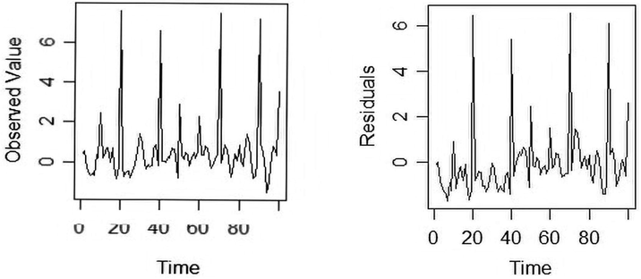

Close

Fig 1

ARMA (2, 2) data contaminated with outliers and its estimated residuals.

Export to PPT

For comparing the performance of the proposed method, some more time series with different set of parameters are simulated. To each simulated time series, outliers are added after a regular interval. The magnitude of the outliers is kept at $4\sigma$ and $5\sigma$. Here $\sigma$ denotes the standard deviation of the time series. Table 1 shows the performance of the proposed algorithm along with other methods.

From Table 1, it can be observed that the performance of the proposed method is better compared to others methods. Performances are compared in terms of correlation of the predicted values with that of originals and SE of predicted errors. The method which is effective in identifying outliers is expected to have lesser SE and higher correlation between predicted and original values.

Data set II: In this case, the following system that represents biological characteristics of single neurons has been considered to simulate nonlinear time series. The set of differential equation discussed below represents the Morris-Lecar (M-L) neural system

In the above model, X represents the membrane potential of the neuronal cell, Y is the activation variable, and Z is the applied input current. The parameter values – $g_{\mathit{Ca}},g_K$ and $g_L$ represent the maximum conductances corresponding to the $C{a}^{+2},K^{+}$ and leak currents, respectively. $V^K$ and $V^L$ represent the reversal potentials corresponding to the above ionic currents. The parameters $V_1,V_2,V_3\text{and}{V}_4$ are appropriately chosen for the hyperbolic functions so that they can attain their equilibrium points instantaneously.

Fourth order Runge-Kutta (RK) method has been used to simulate data for $(X,Y,Z).$Time interval considered in the simulation process is $\mathrm{\Delta }t=0.001$ seconds and simulation is carried out over a time period of 20 s. Simulated time series are presented in Fig 2. Data for these simulated variables are tested for nonlinearity as suggested by Teraesvirta et al. (1993) and the below table presents the result of nonlinearity test.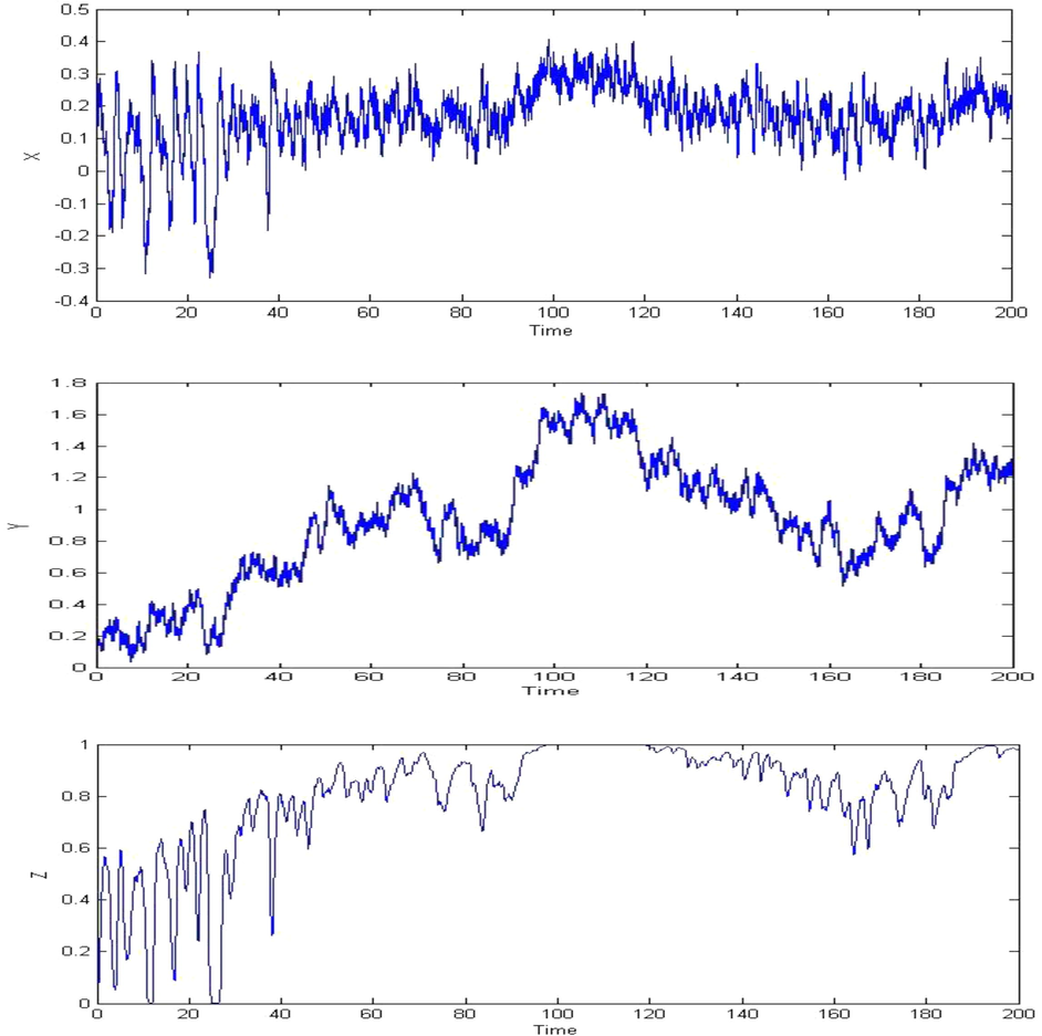

Close

Fig 2

Plot of the time series (X, Y, Z) from the model described in equations (13), (14) and (15).

Export to PPT

Results in Table 2 confirm that X and Y are non-linear in nature. The discussed methods of identifying outliers in a time series are applied to the simulated time series of $(X,Y).$ While 90% of the simulated initial data is used for training, the rest 10% is used for prediction. Correlation of the predicted and actual values along with the SE of the predicted errors is presented in Table 3. The noticeable point here is that, Chen and Liu method does not find any outlier in simulated time series of $X$. However, BARD and OTSAD identifies outliers in both the time series of $X$ and $Y$. The outlier-free data is used for prediction and the result obtained by application of various methods is presented in Table 3.

Data set III: In this case, two time series of TCS stock price and Aluminum trading prices for the period January 2, 2006 to December 31, 2010 and December 24, 2014 to April 12, 2015 are considered respectively. The reason for considering these two time series is to discuss the issue of unusual jumps and drops observed in a financial time series. Generally, in a corporate action such as stock split, a company divides its existing shares into multiple shares. This causes increase in the number of shares by a specific multiple but at the same time the whole value of the shares remains the same. The price of the resulting shares will suddenly drop to half or one third based on split ration. Similar fluctuations are also observed in case of nearing expiry dates of commodity contracts. A contract that will expire after several years from now will remain relatively illiquid until it gets closer to its expiry. As the liquidity increases near the expiry date, sudden change in price of the commodity can be observed. The consequences of these corporate actions may result in the following:

1. The return distribution may change.

2. Most of the outlier detection algorithm may detect the changes in price brought in due to stock split or nearing maturity dates as outlier.

Data for commodity (Aluminum) has been taken from the website http://www.mcxindia.com. Contract expiry dates for the corresponding metal can also be obtained from the same website. The change in price of a financial instrument due to its nearing maturity of stock is not market-driven and brings in unexpected volatility. Leveling such volatility is to smoothen the historical prices of a time series based on the changes brought in due to recent corporate events. The following method of adjustment has been applied to reduce the effect of corporate events on a financial time series.

Let $t_1,t_2,...,t_k$ are the dates of $k$ corporate events of a financial instrument. $\mathrm{\Delta }{p}_i=\{p_{i+1}-p_i\},i=1,2,...,k-1$ is the change in price due to the $i^{\mathit{th}}$ corporate event. Then the method of adjusting historical prices for a financial instrument will be as below

1. Calculate the price change factor at 1st date of corporate event $\mathrm{\Delta }{p}_{t_1}=p_{(t_1+1)}-p_{t_1}$

2. Adjust the historical prices till $(t_2+1)$with change factor $\mathrm{\Delta }{p}_{t_1}.$ Denote adjusted price on $(t_2+1)$ as $p_{(t_2+1)}^{\prime }$ where $p_{(t_2+1)}^{\prime }=p_{(t_2+1)}+\mathrm{\Delta }{p}_{t_1}.$

3. The change factor on date $t_2$ is calculated based on the adjusted price on $(t_2+1)$ day (i.e., $p_{(t_2+1)}^{\prime }$) and actual historical price on $t_2^{\mathit{th}}$ day as $\mathrm{\Delta }{p}_{t_2}=p_{(t_2+1)}^{\prime }-p_{t_2}$

4. Continue the process till the last date of corporate event.

The process of such an adjustment reduces the unwanted volatility in a financial instrument. Table 4 shows the change in volatility level due to the application of the method of the adjustment discussed above.

The changes in price level are also presented graphically in Fig 3. However, question may arise about the need of carrying out such adjustments. The change in price level due to nearing maturity or stock split is such that most of the outlier detecting algorithm will detect such price changes as outliers. Actual outliers may remain in the data for the sake of corporate action and any analysis may come out with fallacious results. Indeed, the proposed adjustment method changes the historical prices relative to the current price level. After adjusting the time series, the proposed method of the outlier detection is applied to both adjusted and original time series, the results of which are presented Table 5. It may be noticed that the efficiency of BARD in some cases is better than the proposed method. The increase in efficiency of BARD is mainly due to the removal of the larger regions from the original data as depicted in Fig 4. The detected regions are presented in a different colour bounded by red lines. From Fig 4 it can be observed that, changes in the level of the data due to stock split and expiry of commodity contract dates are actually identified by BARD as the region of anomalies. However, mere elimination of such region may not be a proper justification. Thus, the method of adjustment discussed above may help in locating actual outliers.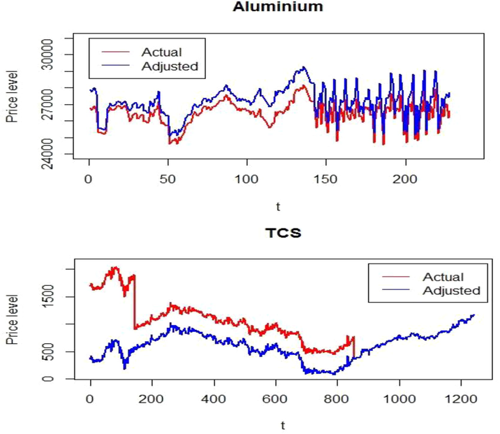

Close

Fig 3

Plot showing the effect of adjustment method on the considered time series (TCS and aluminum).

Export to PPT

Close

Fig 4

Plot showing anomalies region detected by BARD on TCS and aluminum time series.

Export to PPT

6 Conclusion

In the present study, a multivariate outlier detection algorithm has been studied. A univariate time series is transformed to a bivariate data frame based on the robust estimate of lag. Different methods are applied to identify the outliers in time series. Feed forward neural network has been applied to the outlier free time series for model building. Comparison has been carried out based on correlation between predicted and actual values and SE of predicted errors. The discussed method of identifying outliers has been applied to ARMA process as well as to non-linear time series. The efficiency of the proposed algorithm is due to its ability to locate actual outliers unlike BARD and MHD which identify outliers as region and pairs, respectively. The performance of another method OSTAD in identifying outliers has also been compared. The performance of the proposed method is satisfying and may be handy in detecting outliers in time series. In addition, the proposed method does not require a priori knowledge of model parameters. Apart from the simulation examples, time series for TCS share price and commodity price are also considered. However, the proposed method is limited to univariate time series.

Disclosure of any funding to the study

Elsawah received the partially support from UIC Grants (Nos. R201810, R201912 and R202010) and the Zhuhai Premier Discipline Grant to carry out this research work but not for APC.

References

- Unsupervised real-time anomaly detection for streaming data. Neurocomputing. 2017;262:134-147.
- [Google Scholar]
- Bayesian detection of abnormal segments in multiple time series. Bayesian Anal.. 2017;12(1):193-218.
- Outliers in Statistical Data. John Wiley; 1994.
- Statistical methods for outlier detection in space telemetries. In: Space Operations: Inspiring Humankind's Future. Cham: Springer; 2019. p. :513-547.
- Outlier detection and estimation in nonlinear time series. J. Time Ser. Anal.. 2005;26:107-121.
- Analyzing rare event, anomaly, novelty and outlier detection terms under the supervised classification framework. Artif. Intell. Rev. 2019:1-20.
- Estimation of time series parameters in the presence of outliers. Technometrics. 1988;30:193-204.
- Novel algorithms for web software fault prediction. Qual. Reliab. Eng. Int. 2014
- [CrossRef] [Google Scholar]
- Joint estimation of model parameters and outlier effects in time series. J. Am. Stat. Assoc.. 1993;88:284-297.
- Robust estimation of the first-order autoregressive parameter. J. Am. Stat. Assoc.. 1979;88:284-297.
- Effects of a single outlier on ARMA identification. Commun. Stat.-Theory Methods. 1990;19:2207-22027.
- Time series Forecasting with Neural network: a comprehensive study using the airline data. Appl. Stat.. 1998;47:231-250.
- Multivariate outlier detection in exploration geochemistry. Comput. Geosci.. 2005;31:579-587.
- A modification of a method for the detection of outliers in multivariate samples. J. Royal Stat. Soc. Ser. B (Methodol.). 1994;56:393-396.
- Identification of Outliers. Chapman and Hall; 1980.
- Computing the nearest correlation matrix – a problem from finance. IMA J. Numer. Anal.. 2002;22:329-343.
- Approximation capabilities of multilayer feed forward networks. Neural Networks. 1991;4:251-257.
- Multilayer feedforward networks are universal approximators. Neural Networks. 1989;2:359-366.
- Robust Statistics. New York: John Wiley and Sons; 1981.
- Otsad: A package for online time-series anomaly detectors. Neurocomputing. 2020;374:49-53.
- Simultaneous discovery of rare and common segment variants. Biometrika. 2013;100(1):157-172.
- Applied Multivariate Statistical Analysis. Prentice Hall; 1992.
- An artificial neural network (p, d, q) model for time series forecasting. Expert Syst. Appl.. 2010;37:479-489.
- The effect of additive outliers on the forecasts from ARMA models. Int. J. Forecast.. 1989;5:231-240.
- Robust estimation of the scale and of the auto covariance function of Gaussian short and long-range dependent processes. J. Time Ser. Anal.. 2011;32:135-156.
- On-line outlier detection and data cleaning. Comput. Chem. Eng.. 2004;28:1635-1647.
- Kurtosis-based projection pursuit for outlier detection in financial time series. Eur. J. Fin.. 2020;26(2–3):142-164.
- Robust estimation in long-memory processes under additive outliers. J. Stat. Plann. Inference. 2009;139:2511-2525.
- Machine learning techniques for anomaly detection: an overview. Int. J. Comput. Appl.. 2013;79(2):33-37.
- Back propagation neural networks and multiple regressions in the case of heteroscedasticity. Commun. Stat. – Simul. Comput.. 2017;46(9):6772-6789.
- Unmasking multivariate outliers and leverage points. J. Am. Stat. Assoc.. 1990;85(411):633-651.
- A fast algorithm for the minimum covariance determinant estimator. Technometrics. 1999;41:212-223.
- Feedforward neural network based non-linear dynamic modeling of a TRMS using RPROP algorithm. Aircraft Eng. Aerosp. Technol.. 2005;77:13-22.
- Outliers, level shifts, and variance changes in time series. J. Forecasting. 1988;7:1-20.
- Forecasting with artificial neural networks: the state of the art. Int. J. Forecast.. 1998;14:35-62.