

Translate this page into:
Almost unbiased optimum estimators for population mean using dual auxiliary information
⁎Corresponding author. mirfan@gcuf.edu.pk (Muhammad Irfan),
-
Received: ,
Accepted: ,
This article was originally published by Elsevier and was migrated to Scientific Scholar after the change of Publisher.
Peer review under responsibility of King Saud University.
Abstract
One eminent disadvantage of many existing optimal estimators/class of estimators is that they are typically biased. In this article, we proposed an optimum class of unbiased estimators for estimating the population mean under simple random sampling without replacement (SRSWOR) scheme. Proposed class is a blend of three concepts: 1) information on auxiliary variable, 2) the ranks of auxiliary variable and 3) Hartley-Ross type unbiased estimation procedure. Expressions for the bias and the minimum variance of the new class are derived up to first degree of approximation. To highlight the application of proposed class, five real data sets are used. Numerical findings confirm that the new class behaves efficiently as compared to traditional unbiased estimator and other almost unbiased estimators under study. In addition, Monte Carlo simulation study is conducted through two real populations to assess the performance of proposed class against competitors. On the basis of theoretical and numerical findings, it is concluded that new proposed class can generate optimum unbiased estimators under SRSWOR scheme. Therefore, use of proposed class is recommended for future applications.
Keywords
Auxiliary variable
Hartley-Ross type estimator
Ranked auxiliary variable
Unbiased
Variance

1 Introduction
Utilizing the auxiliary information to boost the efficiency of estimators is a common practice in the theory of survey sampling. The auxiliary information such as standard deviation , coefficient of variation, coefficient of skewness , coefficient of kurtosis , coefficient of correlation etc. may play positive role in the selection of sample, strata, type of estimators or in estimation. If this auxiliary information is positively (high) correlated with study variable, ratio estimators are preferred and in case it is negatively (high) correlated, product estimators are used. In this context, some notable contributions were made by Upadhyaya and Singh (1999), Singh and Tailor (2003), Kadilar and Cingi (2006a, 2006b), Gupta and Shabbir (2008), Shabbir and Gupta (2011), Haq and Shabbir (2013), Singh and Solanki (2013), Irfan et al. (2019a, 2019b), Raza et al. (2020) and many others.
Consider a sample of pair of observations ( for the study and auxiliary variables, respectively are selected from a finite population of size under simple random sampling without replacement (SRSWOR) subject to the constraint. Let denotes the ranks of auxiliary variable and denotes the value of in the population. Important measures related to study variable , auxiliary variable and the ranks of auxiliary variable are described in Table 1.
are the unbiased estimators of , respectively.
are also unbiased estimators of respectively.
Similarly,are the unbiased estimators of their population parameters respectively.
2 Unbiased/Almost unbiased estimators from literature
Usually, ratio and product type of estimators of population mean are biased and inconsistent and thus can lead to erroneous inferences. Several researchers have attempted to reduce the bias from these estimators as unbiasedness is one of the important properties of estimators. Unbiased ratio and product type estimators have also been discussed by Hartely and Ross (1954), Robson (1957), Murthy and Nanjamma (1959), Biradar and Singh (1992a, 1992b, 1995), Sahoo et al. (1994) and Javed et al. (2019).
This section presents a comprehensive detail of unbiased/almost unbiased estimators of population mean under simple random sampling scheme from literature.
2.1 Traditional unbiased estimator
The traditional unbiased estimator of population mean along with its variance is
2.2 Hartley and Ross (1954) estimator
Hartley and Ross (1954) suggested an unbiased ratio type estimator for estimating population mean as below
The variance of this estimator, to the first order of approximation, is equal to the mean square error of the usual ratio estimator (see Singh and Mangat (1996)).
2.3 Singh et al. (2014) estimators
Singh et al. (2014) considered the estimators of Kadilar and Cingi (2006c) and Upadhyaya and Singh (1999) to propose the following Hartley-Ross type unbiased estimators for population mean.
here is the coefficient of correlation between study variable and auxiliary variable and is the coefficient of kurtosis of auxiliary variable
Variance of and are respectively given below.
2.4 Cekim and Kadilar (2016) estimators
A general class of Hartley-Ross type unbiased estimators was developed by Cekim and Kadilar (2016) from special version of estimators of Khoshnevisan et al. (2007) as given below
and are either known constants or functions of any known population parameters of auxiliary variable including coefficient of skewness, coefficient of kurtosis, coefficient of variation and coefficient of correlation etc.
Variance of is given as under
It is worth pointing out that if we have
1) and in , then
and
2) and in , then
and
Another class proposed by Cekim and Kadilar (2016) using the special version of Koyuncu and Kadilar (2009) is defined below
is the weight to be determined such that the variance becomes minimum and and are the same as defined earlier.
Differentiating Eq. (12) with respect to and equating to zero, we get the optimal value of as follows
where
Putting the optimal value of in Eq. (12), we get the minimum variance as
3 Methodology
All contributions for efficient estimation of population mean under simple random sampling scheme and alike published work are based on only the utilization of original auxiliary information. None of them tried the dual use of auxiliary information to explore the unbiased estimators for population mean under simple random sampling.
Recently, Irfan et al. (2020) and Javed and Irfan (2020) used an additional information of the auxiliary variable called ranked auxiliary variable to develop efficient estimators under simple and stratified random sampling.
First time, we initiated a blend of three concepts to explore an optimum class of almost unbiased estimators for estimating the population mean:
information on auxiliary variable
the ranks of auxiliary variable
Hartley-Ross type unbiased estimation
A class of biased estimators proposed by Haq et al. (2017) is as follows:
Bias of the class given in Eq. (14) is derived, up to first order of approximation as
Subtracting Eq. (15) from Eq. (14), we obtained the expression given below
After some simplification and replacing the parameters and by their unbiased estimators and in Eq. (16), we have
So, the proposed class of almost unbiased estimators is as follows:
are the suitable weights to be chosen. and are either known constants or functions of any known population parameters of auxiliary variable including coefficient of skewness , coefficient of kurtosis , coefficient of variation and coefficient of correlation etc.
Following are the relative error terms along with their expectations, used to derive the expressions for the bias, variance and minimum variance of the proposed estimators.
such that
In order to obtain the values of , following expressions are helpful.
After rewriting in terms of relative errors and expanding up to first order of approximation, we get
Subtracting from both sides of Eq. (18), we have
Taking expectation on both sides of Eq. (19) to get the
During simplification, all the terms cancel out and we get zero bias which shows that the proposed class generates almost unbiased estimators. As the first order approximation is used in deriving the expression therefore the term “almost” is added here. So,
Squaring both sides of Eq. (19) and taking the expectation, we get the variance of proposed estimators up to first order of approximation as:
where
Partially differentiating Eq. (20) with respect to and and equating them to zero, we get the optimal values of and as follows.
Placing these optimal values in Eq. (20), we obtained the minimum variance as given by
where
4 Results and discussion
In this section, we evaluated the performance of proposed class of estimators as compared to other unbiased/almost unbiased estimators. For this purpose, we selected five real life data sets with different correlation coefficients (first three with positive and last two with negative) between study variable and auxiliary variable. The descriptions of the populations are given below.
Population 1: [Source: Singh and Mangat (1996), p. 369]
Population 2: [Source: Cochran (1977), p.152]
Population 3: [Source: Singh and Mangat (1996), p. 369]
Population 4: [Source: Gujarati (2004), p. 433]
Population 5: [Source: Gujarati (2004), p. 433]
We calculated the variances of all the estimators i.e. for the populations 1–5. Expressions for the variances of all the existing and proposed estimators are given in section 1 & section 3 in detail. All empirical results are summarized in Tables 2-6. *Bold values indicate minimum variances *Bold values indicate minimum variances *Bold values indicate minimum variances *Bold values indicate minimum variances *Bold values indicate minimum variances
Estimator
Variance
Classes of Estimators
1109.534
1
196.0392
152.9700
146.4461
173.4709
1
184.9776
153.2623
146.9481
195.5583
197.5358
152.9325
146.3866
183.1241
195.8957
152.9736
146.4518
197.5143
152.9330
146.3874
184.0929
153.2871
146.9945
165.6300
153.9599
149.1641
1
195.8893
152.9738
146.4521
183.1241
153.3145
147.0466
195.5583
152.9821
146.4655
1
193.0592
153.0459
146.5696
Estimator
Variance
Classes of Estimators
953.8721
1
191.0767
37.6156
16.6971
39.0457
1
60.3292
37.5857
17.4239
194.9164
300.6648
37.5954
16.5412
60.9889
189.4141
37.6160
16.7006
301.8640
37.5952
16.5423
59.3432
37.5826
17.4398
45.8849
36.1171
19.4647
1
193.8267
37.6150
16.6914
60.9889
37.5876
17.4137
194.9164
37.6148
16.6891
1
118.8250
37.6290
16.9256
Estimator
Variance
Classes of Estimators
1109.5340
1
192.3828
207.8877
169.8932
188.2657
1
202.3949
208.5434
171.9661
188.7435
205.5316
207.5081
169.3616
215.0774
191.3648
207.9301
169.9596
204.5481
207.5305
169.3906
206.9720
208.5160
172.1645
211.8509
208.4709
172.3533
1
190.9106
207.9504
169.9920
215.0774
208.4339
172.4686
188.7435
208.0659
170.1863
1
187.1201
208.3344
170.7391
Estimator
Variance
Classes of Estimators
5.0712
1
9.1068
2.6919
2.2790
8.9364
1
8.9279
2.6920
2.2791
9.3860
9.1112
2.6919
2.2790
7.9898
9.1211
2.6919
2.2789
9.1204
2.6919
2.2789
9.4125
2.6917
2.2788
8.9596
2.6920
2.2790
1
9.1451
2.6919
2.2789
7.9898
2.6925
2.2794
9.3859
2.6918
2.2789
1
9.0257
2.6919
2.2790
Estimator
Variance
Classes of Estimators
4.3690
1
10.0399
3.7985
3.3712
9.3363
1
9.9681
3.7984
3.3715
10.2410
10.0379
3.7985
3.3713
9.6624
10.1291
3.7985
3.3709
10.1062
3.7986
3.3710
10.3397
3.7986
3.3703
8.2728
3.7976
3.3778
1
10.1028
3.7985
3.3710
9.6624
3.7984
3.3725
10.2410
3.7986
3.3706
1
10.1266
3.7985
3.3709
In case of positive correlation between study variable and auxiliary variable (populations 1–3), some important observations are made from Tables 2-4 as follows:
performs better than .
It is worth pointing out that has less variance than .
All the proposed estimators have minimum variance as compared to
A deep insight of columns of reveals that the value of provides the least variance among all proposed estimators.
In case of negative correlation between study variable and auxiliary variable (populations 4–5), following important considerations are made from Tables 5-6:
It is perceived that performs better than .
It is important to mention that has less variance than
All proposed estimators have minimum variance as compared to existing estimators.
is an appropriate choice in order to get the minimum variance among all the proposed estimators.
4.1 A simulation study
It is clearly observed from numerical findings that the proposed class provides almost unbiased and efficient estimators for estimating population mean in case of SRSWOR. In addition, this superiority is assessed through a Monte Carlo simulation study using R software. For this purpose, two real populations are used. Different sample sizes i.e. are used for both real populations.
Following steps are performed to carry out the simulation study:
Step 1. Select a SRSWOR of size from the population of size .
Step 2. Use sample data from step 1 to find the variance/minimum variance of all the
existing and proposed estimators.
Step 3. Step 1 and step 2 are repeated 10,000 times.
Step 4. Obtain 10,000 values for variance of each estimator.
Step 5. Average of 10,000 values, obtained in step 4 is the variance of each estimator.
The following expression is used for calculation of variance/minimum variance for all estimators considered in this study:
4.1.1 Real population 1
We used a real data of primary and secondary schools for 923 districts of Turkey in 2007, taking number of teachers as study variable and number of students as auxiliary variable (Source: Koyuncu and Kadilar, 2009). Some important parameters of the data set are:
4.1.2 Real population 2
This real data relates to 81 cars in which average miles per gallons (MPG) is taken as a study variable and top speed, miles per hour (SP) as an auxiliary variable. (Source: Gujarati (2004), p. 433). Some important parameters of the data set are:
Variances calculated for different sample sizes through real populations 1–2 are reported in Tables 7-8. Simulation study, alike in applications to real data reveals that
is more efficient than in case of positive correlation between study variable and auxiliary variable (see Table 7) but less efficient in case of negative correlation (see Table 8).
By increasing the sample size, variance of all the estimators reduces.
Proposed estimators have minimum variance as compared to all other estimators.
| Estimator | Variance | Classes of Estimators | ||||
|---|---|---|---|---|---|---|
| 2510.8720 | 505.7589 | 206.0152 | 178.9120 | |||
| 271.3697 | 478.7737 | 208.0823 | 180.6443 | |||
| 506.8906 | 505.8466 | 204.0754 | 176.6485 | |||
| 490.9651 | 508.3117 | 207.6117 | 180.2311 | |||
| 505.5180 | 207.5761 | 180.9583 | ||||
| 483.6694 | 202.0577 | 175.2135 | ||||
| 229.4068 | 206.3638 | 179.6351 | ||||
| 504.0403 | 208.9553 | 182.3116 | ||||
| 490.9651 | 200.0236 | 173.7984 | ||||
| 506.8906 | 203.3060 | 176.9591 | ||||
| 498.5304 | 203.1903 | 176.5236 | ||||
| 1938.0569 | 390.0107 | 161.6810 | 144.0454 | |||
| 209.1543 | 372.9320 | 162.4285 | 144.7053 | |||
| 393.2290 | 393.0053 | 158.8819 | 141.2770 | |||
| 385.2977 | 390.6282 | 160.2888 | 142.3775 | |||
| 393.9777 | 162.1509 | 144.2795 | ||||
| 373.2435 | 163.9430 | 146.4945 | ||||
| 178.2684 | 159.8451 | 142.1195 | ||||
| 392.5001 | 163.9137 | 146.3558 | ||||
| 385.2977 | 158.3126 | 140.8176 | ||||
| 393.2290 | 160.8272 | 143.2344 | ||||
| 388.8904 | 158.9783 | 141.3371 | ||||
*Bold values indicate minimum variances
| Estimator | Variance | Classes of Estimators | ||||
|---|---|---|---|---|---|---|
| 4.3528 | 7.8021 | 2.0194 | 1.5434 | |||
| 7.7071 | 7.6910 | 2.0369 | 1.5463 | |||
| 8.0659 | 7.8296 | 2.0300 | 1.5328 | |||
| 6.8708 | 7.8169 | 2.0165 | 1.5264 | |||
| 7.8105 | 2.0501 | 1.5596 | ||||
| 8.1228 | 2.0344 | 1.5473 | ||||
| 7.6585 | 2.0146 | 1.5305 | ||||
| 7.8603 | 2.0412 | 1.5490 | ||||
| 6.8708 | 2.0101 | 1.5387 | ||||
| 8.0659 | 2.0610 | 1.5616 | ||||
| 7.7222 | 2.0231 | 1.5402 | ||||
| 3.8208 | 6.8307 | 1.8090 | 1.3954 | |||
| 6.7615 | 6.6893 | 1.7862 | 1.3836 | |||
| 7.0436 | 6.8060 | 1.8016 | 1.4004 | |||
| 5.9986 | 6.8150 | 1.8009 | 1.3975 | |||
| 6.8163 | 1.7871 | 1.3887 | ||||
| 7.0883 | 1.8057 | 1.3974 | ||||
| 6.6915 | 1.7788 | 1.3871 | ||||
| 6.8542 | 1.7990 | 1.3909 | ||||
| 5.9986 | 1.8138 | 1.4053 | ||||
| 7.0436 | 1.8051 | 1.3953 | ||||
| 6.7303 | 1.8095 | 1.3998 | ||||
*Bold values indicate minimum variances
The performance of the proposed estimators as compared to are also shown graphically for both populations considered in simulation study. Figs. 1-2 comprise the average of mean squared errors of the estimators based on different sample sizes. From Figs. 1 & 2, it can be seen that: 1) By increasing the sample size, variance of all the estimators reduces. 2) Proposed estimators have minimum variance as compared to all other estimators under study.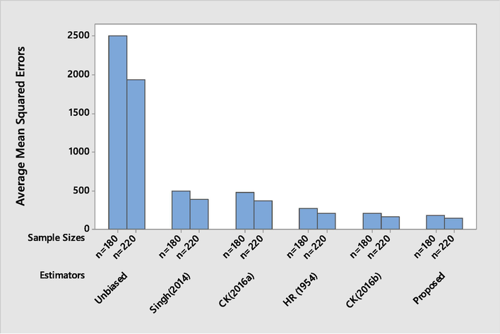
Minimum variance of estimators based on simulation through real population 1.
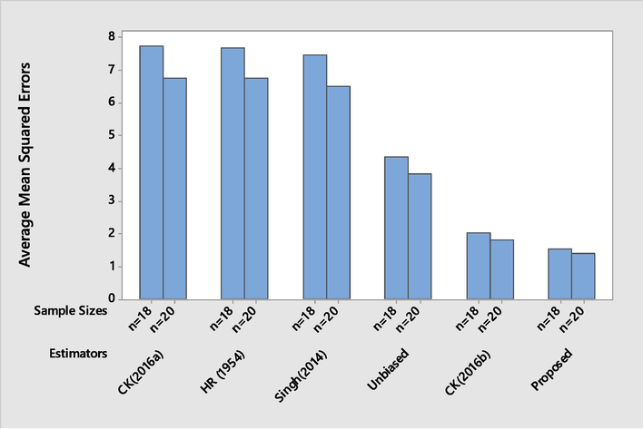
Minimum variance of estimators based on simulation through real population 2.
5 Conclusion
We proposed a new class of almost unbiased estimators for estimating population mean under SRSWOR. This class is developed through the Hartley-Ross type estimation using the information of auxiliary variable and the ranks of auxiliary variable. Minimum variance of proposed class is derived up to first degree of approximation. Five real life data sets are used to check the numerical performance of new estimators. A comparison of new class is made with existing unbiased/almost unbiased estimators. A simulation study through two real data sets is also conducted to assess the potential of suggested class. On the basis of numerical findings, it is concluded that new class can generate optimum almost unbiased estimators. Therefore, use of proposed class is recommended for future applications.
The possible extensions of this work are to estimate the: 1) finite population mean under other sampling designs like stratified random sampling, double sampling, rank set sampling etc. 2) other unknown finite population parameters including median, variance and proportions etc. 3) population mean in the presence of non-sampling errors.
Declaration of Competing Interest
The authors declare that they have no known competing financial interests or personal relationships that could have appeared to influence the work reported in this paper.
References
- A note on almost unbiased ratio-cum-product estimator. Metron. 1992;40(1–2):249-255.
- [Google Scholar]
- A class of unbiased ratio estimators. J. Indian Soc. Agric. Stat.. 1995;47(3):230-239.
- [Google Scholar]
- New unbiased estimators with the help of Hartley-Ross type estimators. Pakistan J. Stat.. 2016;32(4):247-260.
- [Google Scholar]
- Sampling Techniques. New York: John Wiley and Sons; 1977.
- Basic Econometrics. New York: The McGraw-Hill Companies; 2004.
- On improvement in estimating the population mean in simple random sampling. J. Appl. Stat.. 2008;35(5):559-566.
- [Google Scholar]
- A new estimator of finite population mean based on the dual use of the auxiliary in formation. Communications in Statistics- Theory and Methods. 2017;46(9):4425-4436.
- [Google Scholar]
- Improved family of ratio estimators in simple and stratified random sampling. Communications in Statistics- Theory and Methods. 2013;42(5):782-799.
- [Google Scholar]
- Improved estimation of population mean through known conventional and non-conventional measures of auxiliary variable. Iran. J. Sci. Technol., Trans. A: Sci.. 2019;43(4):1851-1862.
- [Google Scholar]
- Enhanced estimation of population mean in the presence of auxiliary information. J. King Saud Univ.- Sci.. 2019;31(4):1373-1378.
- [Google Scholar]
- Irfan, M., Javed, M., & Bhatti, S., H. (2020). Difference-type-exponential estimators based on dual auxiliary information under simple random sampling. Scientia Iranica: Transactions on Industrial Engineering (E), Accepted.
- A simulation study: new optimal estimators for population mean by using dual auxiliary information in stratified random sampling. J. Taibah Univ. Sci.. 2020;14(1):557-568.
- [Google Scholar]
- Hartley-Ross type unbiased estimators of population mean using two auxiliary variables. Scientia Iranica: Trans. Ind. Eng. (E). 2019;26(6):3835-3845.
- [Google Scholar]
- An improvement in estimating the population mean by using the correlation coefficient. Hacettepe J. Math. Stat.. 2006;35(1):103-109.
- [Google Scholar]
- Improvement in estimating the population mean in simple random sampling. Appl. Math. Lett.. 2006;19:75-79.
- [Google Scholar]
- A general family of estimators for estimating population mean using known value of some population parameter(s) Far East Journal of Theoretical Statistics. 2007;22:181-191.
- [Google Scholar]
- Efficient estimators for the population mean. Hacettepe Journal of Mathematics and Statistics. 2009;38(2):217-225.
- [Google Scholar]
- Almost unbiased estimator based on interpenetrating sub-sample estimates. Sankhya. 1959;21:381-392.
- [Google Scholar]
- Raza, M. A., Nawaz, T., & Aslam, M. (2020). On designing CUSUM charts using ratio-type estimators for monitoring the location of normal processes. Scientia Iranica: Transactions on Industrial Engineering (E), Accepted.
- Application of multivariate polykays to the theory of unbiased ratio type estimation. J. Am. Stat. Assoc.. 1957;50:1225-1226.
- [Google Scholar]
- An alternative approach to estimation in two phase sampling using two auxiliary variables. Biometrical Journal. 1994;36:293-298.
- [Google Scholar]
- On estimating finite population mean in simple and stratified random sampling. Communications in Statistics- Theory and Methods. 2011;40(2):199-212.
- [Google Scholar]
- Elements of survey sampling. Norwell, MA: Kluwer Academic Publishers; 1996.
- Hartley-Ross type estimators for population mean using known parameters of auxiliary variate. Communications in Statistics- Theory and Methods. 2014;43:547-565.
- [Google Scholar]
- Use of known correlation coefficient in estimating the finite population means. Stat. Transition. 2003;6(4):555-560.
- [Google Scholar]
- An efficient class of estimators for the population mean using auxiliary information. Comm. Stat.- Theory Meth.. 2013;42:145-163.
- [Google Scholar]
- Use of transformed auxiliary variable in estimating the finite population mean. Biometrical J.. 1999;41(5):627-636.
- [Google Scholar]


