Adequate soliton solutions to the perturbed Boussinesq equation and the KdV-Caudrey-Dodd-Gibbon equation

M.Ali Akbar; Norhashidah Hj. Mohd. Ali; Tasnim Tanjim

doi:10.1016/j.jksus.2020.06.014

View/Download PDF

Buy Reprints

PDF

Translate this page into:

Original article

32 (

); 2777-2785

doi:

10.1016/j.jksus.2020.06.014

Adequate soliton solutions to the perturbed Boussinesq equation and the KdV-Caudrey-Dodd-Gibbon equation

M.Ali Akbar^{^a,^b,⁎}, Norhashidah Hj. Mohd. Ali^{^a}, Tasnim Tanjim^{^b}

aSchool of Mathematical Sciences, Universiti Sains Malaysia, Malaysia

bDepartment of Applied Mathematics, University of Rajshahi, Bangladesh

⁎Corresponding author. ali.akbar@ru.ac.bd (M.Ali Akbar)

Received: 2019-10-24, Accepted: 2020-6-27, Published: 2020-09-01

Disclaimer:
This article was originally published by Elsevier and was migrated to Scientific Scholar after the change of Publisher.

Peer review under responsibility of King Saud University.

Abstract

The perturbed Boussinesq equation and the KdV-Caudrey-Dodd-Gibbon equation describe the characteristics of longitudinal waves in bars, long water waves, plasma waves, quantum mechanics, acoustic waves, nonlinear optics etc. Thus, the mentioned equations are clearly important in their own right. In this article, the modified auxiliary equation technique has been put in use in order to ascertain exact soliton solutions to the stated nonlinear evolution equations (NLEEs). We determine adequate soliton solutions, explicitly, bell-shaped soliton, kink-soliton, periodic-wave, singular-kink, compacton-soliton and other types. These solutions might play an important role in uncovering the underlying context of the physical incidents. It is noteworthy that the executed method is skilled and effective to examine NLEEs, compatible with computer algebra and provides wide-ranging wave solutions. Thus, the study of exact solutions to other NLEEs through the modified auxiliary equation method is prospective and deserves further research.

Keywords

The perturbed Boussinesq equation

The KdV-Caudrey-Dodd-Gibbon equation

Soliton solution

The modified auxiliary equation method

Show Related Articles from PubMed

1 Introduction

In the current era, the nonlinear evolution equations (NLEEs) have been continuously traced to many innovative applications and remarkable progress has been made in the contribution of the exact solutions for nonlinear partial differential equations, which have been a basic concern for both mathematicians and physicists (Yang et al., 2019, Ilie et al., 2018). Thus, the studies of the soliton solutions (Drazin and Johnson, 1989) for NLEEs have ample importance in searching the nonlinear natural events (Akbar et al., 2019). The NLEEs have significant applications in many disciplines, such as, plasma physics, mathematical physics, optical fiber, mathematical chemistry, water wave mechanics, control theory, solid-state physics, meteorology, nonlinear optics, electromagnetic theory, mechanics, chemical kinematics, system identification, biogenetics, etc. Due to the recurrent appearance in various applications in physics, biology, engineering, signal processing, control theory, finance and dynamics, the exact solutions to NLPDEs have attracted the attention of many studies. The exact solutions of NLPDEs play an important role in the study of nonlinear physical phenomena (Liu et al., 2019).

The studies of searching exact solutions to nonlinear equations if exists, and the numerical solutions are very important for understanding the nonlinear tangible events. There are many investigations that provide explicit and numerical solutions for the differential equations to be adopted. Researchers have developed a number of methods in their various studies (Huseyin and Zehra, 2018, Zehra and Turgut, 2015). As for instance, the first integral method (Zhang et al., 2019), the Hirota’s bilinear transformation method (Wang, 2009), the Backlund transform method (Redkina et al., 2019), the exp-function method (Naher et al., 2011), the sine-Gordon equation expansion method (Korkmaz et al., 2020), the Jacobi elliptic function expansion method (Alquran and Jarrah, 2019; Kumar et al., 2019), the Kudryashov method (Alquran et al., 2020; Ali et al., 2019; Alquran et al., 2019a,b ), the unified method (Alquran et al., 2019a,b), the tanh-function method (Jaradat et al., 2018; Alquran and Jaradat, 2019; Irwaq et al., 2018 ), the $(G^{'} / G)$ -expansion method (Alquran and Yassin, 2018; Inan, 2019), the modified extended tanh-function method (Lv et al., 2018), the generalized and improved $(G^{'} / G)$ -expansion method (Naher et al., 2013), the variation of parameters method (Mohyud-Din et al., 2015), the improved $e x p (- φ (ξ))$ -expansion method (Chen et al., 2018), the modified simple equation method (Roshid and Roshid, 2018), the Galerkin method (Abbaszadeh and Dehghan, 2019a, b), the collocation technique (Dehghan and Shokri, 2007), the meshless base numerical technique (Dehghan and Salehi, 2012), the local weak form meshless technique (Abbaszadeh and Dehghan, 2019a, b), the homotopy analysis method (Dehghan et al., 2010; Altaie et al., 2019), the double auxiliary equation method (Moussa et al., 2019), the exponential rational function method (Bekir and Kaplan, 2016), the Riccati equation mapping method (Javeed et al., 2019) etc.

The study of exact solutions of NLEEs has become an outstanding interest and deserves further investigation by mathematicians and physicists. The perturbed Boussinesq equation (BE) and the KdV-Caudrey-Dodd-Gibbon (KdV-CDG) equation arise in long water waves, elasticity for longitudinal waves in bars, plasma waves, quantum mechanics, acoustic wave, nonlinear optics etc. The modified auxiliary equation technique is compatible, effective and provides ample exact soliton solutions in a unique approach. In this article, our objective is to establish broad-ranging, typical, applicable and comprehensive solutions to the formerly declared equations through putting in use of the modified auxiliary equation method.

2 The modified auxiliary equation method

Let us consider the general nonlinear evolution equation

(2.1)

G (v, v_{t}, v_{x}, v_{y}, v_{z}, v_{tt}, v_{tx} \dots) = 0

where

G

is a nonlinear function of

v

’s and

v = v (x, y, z, t)

is the wave function that we have to calculated.

Step 1: We consider the traveling wave variable of the form

(2.2)

v (x, y, z, t) = V (η), η = l x + m y + n z - ω t .

The wave transformation (2.2) modifies the nonlinear partial differential Eq. (2.1) into the subsequent ordinary differential equation (ODE):

(2.3)

Q (V, V^{'}, V^{''}, V^{'''}, \dots) = 0

wherein prime stands for the derivative with respect to

η

Step 2: In accordance with the modified auxiliary equation method, the exact soliton solution of Eq. (2.3) is assumed to be

(2.4)

V (η) = \sum_{j = 0}^{N} A_{j} a^{j g (η)}

where

A_{0}, A_{1}, \dots, A_{N}

are constants to be calculated, such that

A_{N} \neq 0

and

g (η)

is the solution of the nonlinear equation

(2.5)

g^{'} (η) = \frac{1}{\ln a} \{b a^{- g (η)} + c + d a^{g (η)}\} .

Step 3: In order to find the positive integer $N$ appearing in Eq. (2.4), the balancing principle is to be used.

Step 4: Setting the solution (2.4) including (2.5) into equation (2.3) gives a polynomial of $a^{j g (η)}$ , $(j = 0, 1, 2, \dots)$ . Assigning each coefficient of the ensuing polynomial to zero yields a system of over-determined algebraic equations. Unraveling this system of equations, the values of $A_{j}$ , $l$ , $m$ , $n$ , $ω$ etc. can be determined.

Substituting the solutions of $g (η)$ obtained from (2.5) and the values of the constants $A_{i}$ , $b$ , $c$ and $d$ gained in step 4 into the solution (2.4) gives abundant explicit soliton solutions to the general nonlinear evolution Eq. (2.1).

3 Formulation of the soliton solutions

In this section, we establish the typical, pertinent and wide-ranging explicit soliton solutions to the perturbed BE and the KdV-CDG equation by means of the introduced method. We first establish the solutions to the perturbed Boussinesq equation.

3.1

3.1 The perturbed Boussinesq equation

Mathematical models of tangible events related to solitons involve nonlinearity and dispersion (Wazwaz, 2009). In this sub-section, we examine explicit soliton solutions to the strongly perturbed Boussinesq equation which is given by (Ebadi et al., 2012).

(3.1.1)

q_{tt} - k^{2} q_{xx} + p {(q^{2 n})}_{xx} + r q_{xxxx} = β q_{xx} + ρ q_{xxxx}

where

β

represents the coefficient of dissipation and

ρ

is the higher order stabilization term. Solitons are localized waves that propagate without change of their shape and velocity properties and are stable against mutual collisions (Dehghan et al., 2010), i. e. a soliton is a solitary wave that behaves like a particle or elastic. A soliton moves from the asymptotic state at

ξ \to - \infty

to the other asymptotic state at

ξ \to \infty

is localized in

ξ

. Since we are searching for solitary waves in this article, therefore, the used boundary conditions are

u (ξ) \to 0

u' (ξ) \to 0

u^{'' (ξ)} \to 0, \dots

etc. as

ξ \to \pm \infty

. The Boussinesq equation is one of the celebrated nonlinear evolution equations which is an effective shallow water wave model which also serves as a relevant model in many fields of physics. The Boussinesq-type equations are also works as models in many branches of science and engineering. These equations are often used in coastal engineering.

Now, we introduce the travelling wave variable

(3.1.2)

q (x, t) = u (η), η = x - v t .

The wave variable (3.1.2) modifies perturbed Boussinesq equation into the subsequent ODE

(3.1.3)

v^{2} u^{''} - k^{2} u^{''} + p {(u^{2})}^{''} + r u^{''''} = β u^{''} + ρ u^{''''}

where it is assume that

n = 1

. Integrating (3.1.3) twice and considering the integration constants to zero, since we are searching soliton solutions, the equation (3.1.3) turns into

(3.1.4)

{(v}^{2} - k^{2} - β) u + p u^{2} + (r - ρ) u'' = 0 .

The balancing principle between the highest order derivative term $u''$ with the highest power nonlinear term $u^{2}$ , gives $N = 2 .$

Therefore, for $N = 2$ , from (2.4) we obtain the solution of equation (3.1.4) of the form

(3.1.5)

u (η) = A_{0} + A_{1} a^{g (η)} + A_{2} a^{2 g (η)}

where

g (η)

is the solution of the nonlinear Eq. (2.5).

Inserting the solution (3.1.5) and using (2.5) into the equation (3.1.4), with the help of Maple we obtain $a^{4 g (η)} \{p A_{2}^{2} + 6 A_{2} (r - ρ) d^{2}\} + a^{3 g (η)} \{2 p A_{1} A_{2} + 2 (r - ρ) A_{1} d^{2} + 10 (r - ρ) A_{2} c d\} + a^{2 g (η)} \{A_{2} (v^{2} - k^{2} - β) + p A_{1}^{2} + 2 p A_{0} A_{2} + 3 (r - ρ) A_{1} c d + 4 (r - ρ) A_{2} c^{2} + 8 (r - ρ) A_{2} b d\} + \{(v^{2} - k^{2} - β) A_{1} + 2 p A_{0} A_{1} + (r - ρ) A_{1} c^{2} + 2 (r - ρ) A_{1} b d + 6 (r - ρ) A_{2} b c\} a^{g (η)} + {(v^{2} - k^{2} - β) A_{0} + p A_{0}^{2} + (r - ρ) A_{1} b c + 2 {(r - ρ) A}_{2} b^{2}} = 0 .$

Setting the coefficients of $a^{j g (η)} (j = 0, 1, 2, 3, 4)$ to zero leads to the following algebraic system: $p A_{2}^{2} + 6 A_{2} (r - ρ) d^{2} = 0$ $2 p A_{1} A_{2} + 2 (r - ρ) A_{1} d^{2} + 10 (r - ρ) A_{2} c d = 0$ $A_{2} (v^{2} - k^{2} - β) + p A_{1}^{2} + 2 p A_{0} A_{2} + 3 (r - ρ) A_{1} c d + 4 (r - ρ) A_{2} c^{2} + 8 (r - ρ) A_{2} b d = 0$ $(v^{2} - k^{2} - β) A_{1} + 2 p A_{0} A_{1} + (r - ρ) A_{1} c^{2} + 2 (r - ρ) A_{1} b d + 6 (r - ρ) A_{2} b c = 0$ $(v^{2} - k^{2} - β) A_{0} + p A_{0}^{2} + (r - ρ) A_{1} b c + 2 {(r - ρ) A}_{2} b^{2} = 0$

Solving the above algebraic equations with the aid of Maple, we obtain

(3.1.6)

v = \pm \sqrt{- r c^{2} + 4 r d b - 4 ρ d b + β + ρ c^{2} + k^{2}}, A_{0} = - \frac{6 d b (r - ρ)}{p}, A_{1} = - \frac{6 d c (r - ρ)}{p}, A_{2} = - \frac{6 d^{2} (r - ρ)}{p}

and $v = \pm \sqrt{r c^{2} - 4 r d b + 4 ρ d b + β - ρ c^{2} + k^{2}}$ , $A_{0} = - \frac{r c^{2} + 2 r d b - 2 ρ d b - ρ c^{2}}{p}$ ,

(3.1.7)

A_{1} = - \frac{6 c d (r - ρ)}{p}, A_{2} = - \frac{6 d^{2} (r - ρ)}{p} .

Now, we will make use the values of the constants scheduled in (3.1.6) and (3.1.7) and the solutions $g (η)$ of the Eq. (2.5) obtained for different constraints on the involved parameters.

Case 1: When $c^{2} - 4 b d < 0$ and $d \neq 0$ , using the values scheduled in (3.1.6), from solution (3.1.5) we attain

(3.1.8)

u (η) = \frac{3 (r - ρ)}{2 p} (c^{2} - 4 b d) \sec^{2} (\frac{\sqrt{4 b d - c^{2}}}{2} η)

And

(3.1.9)

u (η) = \frac{3 (r - ρ)}{2 p} (c^{2} - 4 b d) \csc^{2} (\frac{\sqrt{4 b d - c^{2}}}{2} η) .

On the other hand, using the values scheduled in (3.1.7), from solution (3.1.5) we attain

(3.1.10)

u (η) = \frac{(r - ρ) (c^{2} - 4 b d)}{2 p} \{1 + 3 \tan^{2} (\frac{\sqrt{4 b d - c^{2}}}{2} η)\}

and

(3.1.11)

u (η) = \frac{(r - ρ) (c^{2} - 4 b d)}{2 p} \{1 + 3 \cot^{2} (\frac{\sqrt{4 b d - c^{2}}}{2} η)\} .

Case 2: When $c^{2} - 4 b d > 0$ and $d \neq 0$ , by means of the values assembled in (3.1.6), from solution (3.1.5) we obtain

(3.1.12)

u (η) = \frac{3 (r - ρ) (c^{2} - 4 b d)}{2 p} {sech}^{2} (\frac{\sqrt{c^{2} - 4 b d}}{2}, η)

And

(3.1.13)

u (η) = - \frac{3 (r - ρ) (c^{2} - 4 b d)}{2 p} {csch}^{2} (\frac{\sqrt{c^{2} - 4 b d}}{2}, η) .

Furthermore, by means of the values assembled in (3.1.7), from solution (3.1.5) we obtain

(3.1.14)

u (η) = \frac{(r - ρ) (c^{2} - 4 b d)}{2 p} \{1 - 3 \tanh^{2} (\frac{\sqrt{c^{2} - 4 b d}}{2} η)\}

and

(3.1.15)

u (η) = \frac{(r - ρ) (c^{2} - 4 b d)}{2 p} \{1 - 3 \coth^{2} (\frac{\sqrt{c^{2} - 4 b d}}{2} η)\}

Case 3: When $c^{2} + 4 b^{2} < 0$ , $d \neq 0$ and $d = - b$ , inserting the values of the parameters arranged in (3.1.6), the solution (3.1.5) becomes

(3.1.16)

u (η) = \frac{3 (r - ρ) (c^{2} + 4 b^{2})}{2 p} \sec^{2} \{\frac{\sqrt{- (c^{2} + 4 b^{2})}}{2} η\}

(3.1.17)

u (η) = \frac{3 (r - ρ) (c^{2} + 4 b^{2})}{2 p} \csc^{2} \{\frac{\sqrt{- (c^{2} + 4 b^{2})}}{2} η\} .

Again, inserting the values of the parameters arranged in (3.1.7), the solution (3.1.5) becomes

(3.1.18)

u (η) = \frac{(r - ρ) (c^{2} + 4 b^{2})}{2 p} \{1 + 3 \tan^{2} (\frac{\sqrt{- (c^{2} + 4 b^{2})}}{2} η)\}

and

(3.1.19)

u (η) = \frac{(r - ρ) (c^{2} + 4 b^{2})}{2 p} \{1 + 3 \cot^{2} (\frac{\sqrt{- (c^{2} + 4 b^{2})}}{2} η)\} .

Case 4: When $c^{2} + 4 b^{2} > 0$ , $d \neq 0$ and $d = - b$ , making use of values organized in (3.1.6), from (3.1.5) we achieve

(3.1.20)

u (η) = \frac{(r - ρ) (3 c^{2} + 12 b^{2})}{2 p} {sech}^{2} (\frac{\sqrt{c^{2} + 4 b^{2}}}{2} η)

and

(3.1.21)

u (η) = - \frac{(r - ρ) (3 c^{2} + 12 b^{2})}{2 p} {csch}^{2} (\frac{\sqrt{c^{2} + 4 b^{2}}}{2} η) .

On the contrary, making use of values organized in (3.1.7), from (3.1.5) we achieve the subsequent solution

(3.1.22)

u (η) = \frac{(r - ρ) (c^{2} + 4 b^{2})}{2 p} \{1 - 3 \tanh^{2} (\frac{\sqrt{c^{2} + 4 b^{2}}}{2} η)\}

and

(3.1.23)

u (η) = \frac{(r - ρ) (c^{2} + 4 b^{2})}{2 p} \{1 - 3 \coth^{2} (\frac{\sqrt{c^{2} + 4 b^{2}}}{2} η)\} .

Case 5: When $c^{2} - 4 b^{2} < 0$ and $d = b$ , plugging in the parameters set out in (3.1.6), into solution (3.1.5), we derive

(3.1.24)

u (η) = \frac{3 (r - ρ) (c^{2} - 4 b^{2})}{2 p} \sec^{2} (\frac{\sqrt{- (c^{2} - 4 b^{2})}}{2} η)

and

(3.1.25)

u (η) = \frac{3 (r - ρ) (c^{2} - 4 b^{2})}{2 p} \csc^{2} (\frac{\sqrt{- (c^{2} - 4 b^{2})}}{2} η) .

Alternatively, plugging in the parameters set out in (3.1.7), into solution (3.1.5), we derive

(3.1.26)

u (η) = \frac{(r - ρ) (c^{2} - 4 b^{2})}{2 p} \sec^{2} (\frac{\sqrt{- (c^{2} - 4 b^{2})}}{2} η)

and

(3.1.27)

u (η) = \frac{(r - ρ) (c^{2} - 4 b^{2})}{2 p} \csc^{2} (\frac{\sqrt{- (c^{2} - 4 b^{2})}}{2} η) .

Case 6: When $c^{2} - 4 b^{2} > 0$ and $d = b$ , putting the values of the unknown constants presented in (3.1.6), the solution (3.1.5) developed into

(3.1.28)

u (η) = \frac{3 (r - ρ) (c^{2} - 4 b^{2})}{2 p} {sech}^{2} (\frac{\sqrt{c^{2} - 4 b^{2}}}{2} η)

and

(3.1.29)

u (η) = - \frac{3 (r - ρ) (c^{2} - 4 b^{2})}{2 p} {csch}^{2} (\frac{\sqrt{c^{2} - 4 b^{2}}}{2} η) .

Moreover, putting the values of the unknown constants presented in (3.1.7), the solution (3.1.5) developed into

(3.1.30)

u (η) = \frac{(r - ρ) (c^{2} - 4 b^{2})}{2 p} \{1 - {3 \tanh}^{2} (\frac{\sqrt{c^{2} - 4 b^{2}}}{2} η)\}

And

(3.1.31)

u (η) = \frac{(r - ρ) (c^{2} - 4 b^{2})}{2 p} \{1 - {3 \coth}^{2} (\frac{\sqrt{c^{2} - 4 b^{2}}}{2} η)\} .

Case 7: When $c^{2} = 4 b d$ , putting in use the values of the unknown constants sorted out in (3.1.6) into solution (3.1.5), we ascertain

(3.1.32)

u (η) = - \frac{6 (r - ρ)}{η^{2} p} .

On the other hand, if we put the values of the unknown constants sorted out in (3.1.7) into (3.1.5), we ascertain the solution identical to the solution (3.1.32). But, since there is no different meaning in writing the same solution repeatedly, it has not been written down.

Case 8: When $bd < 0$ , $c = 0$ and $d \neq 0$ , placing the constants displayed in (3.1.6) into solution (3.1.5), we determine

(3.1.33)

u (η) = - \frac{6 d b (r - ρ)}{p} {sech}^{2} (\sqrt{- d b} η)

and

(3.1.34)

u (η) = \frac{6 d b (r - ρ)}{p} {csch}^{2} (\sqrt{- d b} η) .

As opposed to, placing the constants displayed in (3.1.7) into solution (3.1.5), we determine the subsequent solutions

(3.1.35)

u (η) = - \frac{2 d b (r - ρ)}{p} {1 - 3 \tanh^{2} (\sqrt{- d b} η)}

and

(3.1.36)

u (η) = - \frac{2 d b (r - ρ)}{p} \{1 - 3 \coth^{2} (\sqrt{- d b} η)\} .

Case 9: When $c = 0$ and $b = - d$ ,

By means of the values of the parameters gathered in (3.1.6), from solution (3.1.5), we achieve the rational solution

(3.1.37)

u (η) = - \frac{24 d^{2} (r - ρ) e^{(- 2 d η)}}{p {\{- 1 + e^{(- 2 d η)}\}}^{2}}

Making use of values of the constants compiled in (3.1.7) into solution Eq. (3.1.5), we achieve the rational solution

(3.1.38)

u (η) = - \frac{4 d^{2} (r - ρ) \{e^{(- 4 d η)} + 4 e^{(- 2 d η)} + 1\}}{p {\{- 1 + e^{(- 2 d η)}\}}^{2}} .

Case 10: When $c = d = K$ and $b = 0$ , by means of the values amassed in (3.1.6), from Eq. (3.1.5), we accomplish the next exponential solution

(3.1.39)

u (η) = - \frac{6 K^{2} (r - ρ) e^{K η}}{p {(1 - e^{K η})}^{2}}

Also, by means of the values amassed in (3.1.7), from equation (3.1.5), we accomplish the next exponential solution

(3.1.40)

u (η) = - \frac{K^{2} (r - ρ)}{p} - \frac{6 K^{2} (r - ρ) e^{K η}}{p {(1 - e^{K η})}^{2}}

Case 11: When $c = b + d$ , for the values of the parameters accumulated in (3.1.6) into solution equation (3.1.5), we find out the ensuing solution

(3.1.41)

u (η) = - \frac{6 d (r - ρ) {(b - d)}^{2} e^{(b - d) η}}{p {\{1 - d e^{(b - d) η}\}}^{2}}

Similarly, for the values of the parameters accumulated in (3.1.7) into solution equation (3.1.5), we find out the ensuing solution

(3.1.42)

u (η) = - \frac{(r - ρ) (b^{2} + d^{2} + 4 b d)}{p} + \frac{6 d (r - ρ) \{1 - b e^{(b - d) η}\} \{b + 2 d - 2 b d e^{(b - d) η} - d^{2} e^{(b - d) η}\}}{p {\{1 - d e^{(b - d) η}\}}^{2}}

Case 12: When $c = - (b + d)$ , for the estimations of the parameters aggregated in (3.1.6) from solution (3.1.5), we discover the resulting solution

(3.1.43)

u (η) = - \frac{6 d (r - ρ) {(b - d)}^{2} e^{(b - d) η}}{p {\{d - e^{(b - d) η}\}}^{2}}

Again, for the estimations of the parameters aggregated in (3.1.7) from solution (3.1.5), we discover the resulting solution

(3.1.44)

u (η) = - \frac{(r - ρ) (b^{2} + d^{2} + 4 b d)}{p} + \frac{6 d (r - ρ) \{b + e^{(b - d) η}\} \{d^{2} - b e^{(b - d) η}\}}{p {\{d - e^{(b - d) η}\}}^{2}}

Case 13: When $b = 0$ , embeding the values of the constants from (3.1.6) into (3.1.5), we reach

(3.1.45)

u (η) = - \frac{6 d c^{2} (r - ρ) e^{c η}}{p {(1 - d e^{c η})}^{2}}

Likewise, embeding the values of the constants from (3.1.7) into (3.1.5), we reach

(3.1.46)

u (η) = - \frac{c^{2} (r - ρ)}{p} \{\frac{1 + 4 d e^{c η} + d^{2} e^{2 c η}}{{(1 - d e^{c η})}^{2}}\}

Case 14: When $d = c = b \neq 0$ , by means of (3.1.6), from solution (3.1.5) we attain

(3.1.47)

u (η) = - \frac{9 b^{2} (r - ρ)}{2 p} \sec^{2} (\frac{\sqrt{3}}{2} b η) .

Equivalently, by means of (3.1.7), from solution (3.1.5) we attain

(3.1.48)

u (η) = - \frac{3 b^{2} (r - ρ)}{2 p} \{1 + 3 \tan^{2} (\frac{\sqrt{3}}{2} b η)\}

Case 15: When $b = c = 0$ , plugging the values from (3.1.6) into (3.1.5), we extract

(3.1.49)

u (η) = - \frac{6 (r - ρ)}{η^{2} d}

In the similar fashion, if we set the values of the unknown constants sorted out in (3.1.7) into solution (3.1.5), we obtain the same solution (3.1.49). But, since there is no different meaning in writing the same solution recurrently, the solution has not been documented.

Case 16: When $d = b$ and $c = 0$ , putting the values presented in (3.1.6) into equation (3.1.5), we accomplish

(3.1.50)

u (η) = - \frac{6 b^{2} (r - ρ)}{p} \sec^{2} (b η)

Moreover, putting the values presented in (3.1.7) into equation (3.1.5), we accomplish

(3.1.51)

u (η) = - \frac{2 b^{2} (r - ρ)}{p} [1 + {3 \tan}^{2} (b η)]

It is inspected that, by means of the modified auxiliary equation method, we accomplish ample closed form soliton solutions to the perturbed BE which might be worthwhile to analyse the intricate phenomena in science and engineering.

3.2

3.2 The KdV-Caudrey-Dodd-Gibbon equation

In this sub-section, we will extract the closed form soliton solutions to the KdV-CDG equation which might be supportive to portrait the properties of the plasma waves, quantum mechanics, acoustic wave and nonlinear optics through the modified auxiliary equation method. The combined KdV-CDG equation (Biswas et al., 2013) is

(3.2.1)

u_{t} + k {(u_{xx} + \frac{1}{5} α u^{2})}_{x} + p {(\frac{1}{15} α u^{3} + α u u_{xx} + u_{xxxx})}_{x} = 0

It is noted that the KdV-CDG equation plays a significant role in nonlinear science, for example, in plasma physics, laser optics and ocean dynamics (Tu et al., 2016). In this study, the used boundary conditions are $u (ξ) \to 0$ , $u' (ξ) \to 0$ , $u^{'' (ξ)} \to 0, \dots$ etc. as $ξ \to \pm \infty$ , since we are looking for soliton solutions and solitons are localized waves that propagate without change of their shape and velocity properties and are stable against mutual collisions (Dehghan et al., 2010).

Now we introduce the following wave transformation

(3.2.2)

u (x, t) = u (η), η = x - v t .

Using the wave transformation (3.2.2) into equation (3.2.1), it transforms into the following ODE

(3.2.3)

- v u^{'} + k {(u^{''} + \frac{1}{5} α u^{2})}^{'} + p {(\frac{1}{15} α u^{3} + α u u^{''} + u^{''''})}^{'} = 0

Since, we are searching for soliton solutions, integrating equation (3.2.3) and considering the constant of integration to zero, we ascertain

(3.2.4)

- v u + k (u^{''} + \frac{1}{5} α u^{2}) + p (\frac{1}{15} α u^{3} + α u u^{''} + u^{''''}) = 0

The homogeneous balance between the highest order linear term $u''''$ and the nonlinear term highest order $u^{3}$ , yields $N = 2 .$

Therefore, the solution structure of equation (3.2.4) is identical to the solution (3.1.5). Therefore, the shape of the solution has not been rewritten in this section.

Inserting (3.1.5) along with (2.5) into solution (3.2.4) with the help of symbolic computation software Maple, we get a polynomial of $a^{j g (η)}$ . We equate the coefficients of this polynomial to zero and this equalization generates a system of algebraic equations that contains seven equations. For simplicity, we have been avoided to show them. Solving this system of algebraic equations, we attain subsequent set of solutions of the constants

(3.2.5)

v = 16 p d^{2} b^{2} + p c^{4} + k c^{2} - 8 p c^{2} d b - 4 k d b, α = 1, A_{0} = - 30 d b, A_{1} = - 30 c d, A_{2} = - 30 d^{2}

Now, we will look into the closed form soliton solution to the KdV-CDG equation for the values of the constants assembled above together with the values of $a^{g (η)}$ .

Case 1: When $c^{2} - 4 b d < 0$ and $d \neq 0$ , inserting the values of unknown constants arranged in (3.2.5) and from solution (3.1.5), we achieve

(3.2.6)

u (η) = (\frac{15 c^{2}}{2} - 30 bd) \sec^{2} (\frac{\sqrt{4 b d - c^{2}}}{2} η)

And

(3.2.7)

u (η) = {(\frac{15 c^{2}}{2} - 30 b d) c s c}^{2} (\frac{\sqrt{4 b d - c^{2}}}{2} η)

Case 2: When $c^{2} - 4 b d > 0$ and $d \neq 0$ , putting the parameters assorted in (3.2.5) into solution (3.1.5), we attain

(3.2.8)

u (η) = (\frac{15 c^{2}}{2} - 30 b d) {sech}^{2} (\frac{\sqrt{c^{2} - 4 b d}}{2} η)

And

(3.2.9)

u (η) = (30 b d - \frac{15 c^{2}}{2}) {c s c h}^{2} (\frac{\sqrt{c^{2} - 4 b d}}{2}, η)

Case 3: When $c^{2} + 4 b^{2} < 0$ , $d \neq 0$ and $d = - b$ , by means of the constants assembled in (3.2.5) into solution (3.1.5), we accomplish

(32.10)

u (η) = (\frac{15}{2} c^{2} + 30 b^{2}) \sec^{2} (\frac{\sqrt{- c^{2} - 4 b^{2}}}{2} η)

And

(32.11)

u (η) = (\frac{15}{2} c^{2} + 30 b^{2}) \csc^{2} (\frac{\sqrt{- c^{2} - 4 b^{2}}}{2} η)

Case 4: When $c^{2} + 4 b^{2} > 0$ , $d \neq 0$ and $d = - b$ , setting the values of the parameters organized in (3.2.5) into (3.1.5), we ascertain

(32.12)

u (η) = (\frac{15 c^{2}}{2} + 30 b^{2}) {sech}^{2} (\frac{\sqrt{c^{2} + 4 b^{2}}}{2} η)

And

(32.13)

u (η) = - (\frac{15 c^{2}}{2} + 30 b^{2}) {csch}^{2} (\frac{\sqrt{c^{2} + 4 b^{2}}}{2} η)

Case 5: When $c^{2} - 4 b^{2} < 0$ and $d = b$ , making use of (3.2.5), from solution equation (3.1.5), we a reach to the following solutions

(32.14)

u (η) = (\frac{15 c^{2}}{2} - 30 b^{2}) \sec^{2} (\frac{\sqrt{- (c^{2} - 4 b^{2})}}{2} η)

And

(32.15)

u (η) = (\frac{15 c^{2}}{2} - 30 b^{2}) \csc^{2} (\frac{\sqrt{- (c^{2} - 4 b^{2})}}{2} η)

Case 6: When $c^{2} - 4 b^{2} > 0$ and $d = b$ , utilizing (3.2.5), from solution equation (3.1.5), we acquire the under mentioned solutions

(32.16)

u (η) = - (30 b^{2} - \frac{15 c^{2}}{2}) {sech}^{2} (\frac{\sqrt{c^{2} - 4 b^{2}}}{2} η)

And

(32.17)

u (η) = {(30 b^{2} - \frac{15 c^{2}}{2}) csch}^{2} (\frac{\sqrt{c^{2} - 4 b^{2}}}{2} η)

Case 7: When $db < 0$ , $c = 0$ and $d \neq 0$ , substituting (3.2.5) into solution equation (3.1.5), we secure the afterward solutions

(32.18)

u (η) = - 30 d b {sech}^{2} (\sqrt{- d b} η)

And

(32.19)

u (η) = 30 d b {csch}^{2} (\sqrt{- d b} η)

Case 8: When $c = 0$ and $b = - d$ , using (3.2.5), from solution (3.1.5), we derive the exponential solution

(32.20)

u (η) = - \frac{120 d^{2} e^{- 2 d η}}{1 + e^{- 4 d η} - 2 e^{- 2 d η}}

Case 9: When $c = d = K$ and $b = 0$ , embedding (3.2.5) into solution (3.1.5), we determine the next exponential solution

(32.21)

u (η) = - \frac{30 K^{2} e^{K η}}{{(1 - e^{K η})}^{2}}

Case 10: When $c = b + d$ , putting in use (3.2.5) into solution formula (3.1.5), we find out succeeding exponential solution

(32.22)

u (η) = - \frac{30 d {(b - d)}^{2} e^{(b - d) η}}{{\{1 - d e^{(b - d) η}\}}^{2}}

Case 11: When $c = - (b + d)$ , placing (3.2.5) into (3.1.5), we get

(32.23)

u (η) = - \frac{30 d {(b - d)}^{2} e^{(b - d) η}}{{\{d - e^{(b - d) η}\}}^{2}}

Case 12: When $b = 0$ , by means of (3.2.5) from (3.1.5), we derive

(32.24)

u (η) = - \frac{30 c^{2} d e^{c η}}{{(1 - d e^{c η})}^{2}}

Case 13: When $d = c = b \neq 0$ , using (3.2.5) in place of the unrevealed constants containing the solution (3.1.5), we gain

(32.25)

u (η) = - \frac{45}{2} b^{2} \sec^{2} (\frac{\sqrt{3}}{2} b η)

Case 14: When $d = b$ and $c = 0$ , applying (3.2.5) from solution formula (3.1.5), we carry out the following solution

(32.26)

u (η) = - 30 b^{2} {s e c}^{2} (b η)

It is noteworthy that scores of closed form soliton solutions, including bell-shaped soliton, kink-soliton, periodic-wave, singular-kink, compacton-soliton and other types of soliton solutions have been extracted to the KdV-CDG equation that may be suitable for analysing the concerning nonlinear physical phenomena.

4 Graphical representation of the solutions and discussion

In this section, we have depicted some 3D graphs of the achieved solutions of the perturbed BE and the KdV-CDG equation by using symbolic computation software Mathematica in order to visualize the shape and to comprehend tangible events concerning the phenomena.

4.1

4.1 The perturbed Boussinesq equation

Solution (3.1.8) represents singular periodic wave for the values $c = 1$ , $b = 2$ , $d = 3$ , $k = - 2$ , $p = - 2$ , $r = - 1.83$ , $β = - 2$ , $ρ = - 2$ of the parameters and shown in Fig. 1. Periodic travelling waves play an important role in different tangible incidents, including self-reinforcing systems, impulsive systems, reaction–diffusion-advection systems etc. The 3D figure is sketched within the interval 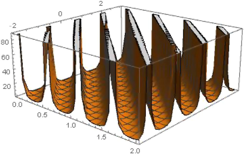$- 2 \leq x \leq 3$ and $0 \leq t \leq 2$ .

3D plot of solution (3.1.8) for c=1, b=2, d=3, k=-2, p=-2, r=-1.83, β=-2 and ρ=-2.

For the values $c = 3$ , $b = - 1$ , $d = 1$ , $k = - . 5$ , $p = - 2$ , $r = - 2$ , $β = - 2$ , $ρ = - 1$ , the solution (3.1.12) represents bell-shape soliton which is characterized by infinite tails or infinite wings and displayed in Fig. 2. The 3D figure is depicted within the interval 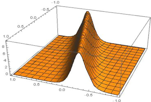$- 1 \leq x, t \leq 2$ .

3D plot of solution (3.1.12) for c=3, b=-1, d=1, k=-.5, p=-2, r=-2, β=-2 and ρ=-1.

Solution (3.1.13) represents singular bell-shape soliton for the values $b = 1$ , $c = 3$ , $d = 2$ , $ρ = 1$ , $β = 1$ , $r = 2$ , $p = 1$ , $k = 1$ of the parameters and portrayed in Fig. 3. Singular solitons are another sort of solitary waves that appear with a singularity, usually infinite discontinuity (Wazwaz 2009). Singular solitons can be connected to solitary waves when the center position of the solitary wave is imaginary (Drazin and Johnson 1989). The 3D figure is plotted within the interval 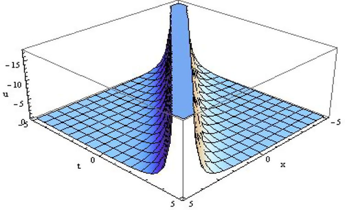$- 5 \leq x, t \leq 5$ .

3D plot of solution (3.1.13) for the values b=1, c=3, d=2, ρ=1, β=1, r=2, p=1 and k=1.

Solution (3.1.38) is a spike like singular soliton for $c = 0$ , $b = - d$ , $d = - 2$ , $k = . 5$ , $p = 1.2$ , $r = 1.25$ , $β = - 1$ , $ρ = - 2$ and documented in Fig. 4. Spike soliton can probably provide an explanation to the formation of Rogue waves. The 3D figure is portrayed within the limit $- 4 \leq x \leq 4$ , $0 \leq t \leq 3$ .

3D plot of solution (3.1.38) for c=0, b=-d, d=-2, k=.5, p=1.2, r=1.25, β=-1 and ρ=-2.

Solution (3.1.39) is an anti-bell shape soliton for the values $c = 0$ , $b = 0$ , $k = 2$ , $d = 1$ , $r = 4$ , $β = 1$ , $ρ = 3$ of the parameters and traced in Fig. 5. The 3D figure is delineated within the interval 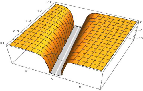$- 8 \leq x \leq 8$ and $0 \leq t \leq 2$ .

3D plot of solution (3.1.39) for c=0, b=0, k=2, d=1, r=4, β=1 and.ρ=3

It is observed from the solutions of the perturbed BE that, the solutions (3.1.8)–(3.1.11), (3.1.16)–(3.1.19), (3.1.24)–(3.1.27), (3.1.30), (3.1.31), (3.1.47), (3.1.48), (3.1.50) and (3.1.51) represent the nature of singular periodic wave. The solutions (3.1.12), (3.1.14), (3.1.28), (3.1.33) and (3.1.35) represent the bell-shape soliton. The solutions (3.1.13), (3.1.15), (3.1.20)–(3.1.23), (3.1.29), (3.1.32), (3.1.34), (3.1.36)–(3.1.38), (3.1.39)–(3.1.41), (3.1.43), (3.1.45), (3.1.46), (3.1.49) and (3.1.50) represent the characteristic of singular bell-shape soliton. The type of the solutions (3.1.42) and (3.1.44) is singular kink soliton.

4.2

4.2 The KdV-Caudrey-Dodd-Gibbon equation

In this subsection, we have portrayed the graphical significance of the results obtained from the KDV-CDG equation for different values of parameters. The 3D graphs of the solutions are shown given:

The solution (3.2.6) is singular periodic wave for the values $c = 1$ , $b = 0.5$ , $d = 1$ , $k = - 2$ , $p = - 2$ of the parameters and specified in Fig. 6. Periodic travelling waves play an important role in self-reinforcing systems, reaction–diffusion-advection systems, impulsive systems etc. The 3D figure is delineated within the interval 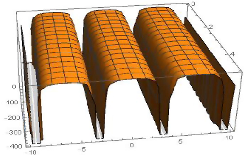$- 10 \leq x \leq 10$ , $0 \leq t \leq 5$ .

3D plot of solution (3.2.6) for c=1, b=0.5, d=1, k=-2 and p=-2.

Solution (32.22) is a compacton soliton for the values $b = - 1.7$ , $d = 0$ , $c = - 1.1$ , $k = 0.2$ , $p = - 2$ of the parameters and indicated in Fig. 7. A compacton is a solitary wave with compact support in which the nonlinear dispersion confines it to a finite core, therefore the exponential wings vanish. The 3D figure is shown within the limit 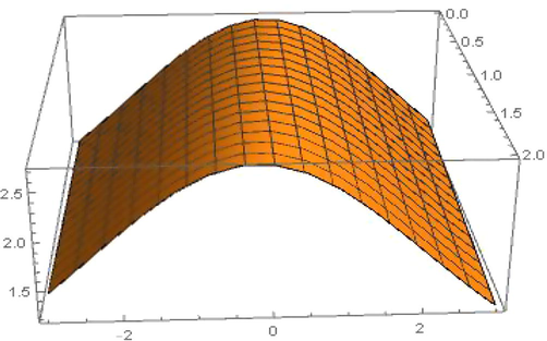$- 3 \leq x \leq 3$ , $0 \leq t \leq 2$ .

3D plot of solution (32.22) for b=-1.7, d=0, c=-1.1, k=0.2 and p=-2.

Solution (32.23) is a singular kink soliton for the values $b = 0$ , $c = 1$ , $d = 1$ , $p = 1$ , $k = 1$ of the constants and presented in Fig. 8. The 3D figure is outlined within the limit 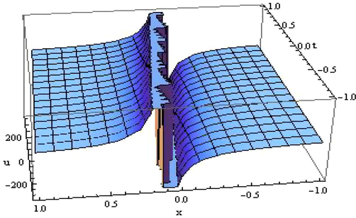$- 10 \leq x, t \leq 10$ .

3D graph of solution (32.23) for the values b=0, c=1, d=1, p=1 and k=1.

Solution (32.24) is a bell-shape soliton for the values $c = - 0.6$ , $b = 0$ , $d = - 1.1$ , $k = - 0.5$ , $p = - 0.6$ of the constants which has infinite wings and plotted in Fig. 9. The 3D figure is outlined within the limit 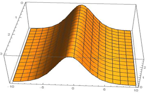$- 10 \leq x \leq 10$ and $0 \leq t \leq 3$ .

3D plot of solution (32.24) for c=-0.6, b=0, d=-1.1, =-0.5 and p=-0.6.

We assert that the obtained solutions might be supportive in analyzing the waves of nonlinear optics, long water waves, plasma waves, quantum mechanics, elasticity for longitudinal waves in bars, acoustic waves etc.

5 Conclusion

In this article, we have extracted scores of closed form soliton solutions to the perturbed Boussinesq equation and the KdV-Caudrey-Dodd-Gibbon equation including bell-shaped soliton, kink-soliton, periodic-wave, singular-kink, compacton-soliton and other types of solitons associated with several free parameters. These free parameters have important implications, such as setting different values of the free parameters from an individual solution cognizant solutions can be found in a unique way. It is valuable to mentioned that the solutions of the NLEEs are achieved in terms of trigonometric, hyperbolic, rational and exponential functions. Some of the obtained solutions are new and thus could be effective in the study of nonlinear physical phenomena. It can be concluded that the adopted method is reliable, effective, conformable and provide ample compatible solutions to NLEEs arise in mathematical physics, applied mathematics and engineering.

Acknowledgements

The authors would like to express their sincere thanks to the anonymous referees for their valuable comments and suggestions to improve the article. This work is supported by the USM Research University Grant 1001/PMATHS/8011016 and the authors acknowledge this support.

Declaration of Competing Interest

The authors declare that they have no known competing financial interests or personal relationships that could have appeared to influence the work reported in this paper.

References

Abbaszadeh M., Dehghan M.. The interpolating element-free Galerkin method for solving Korteweg-de Vries-Rosenau-regularized long-wave equation with error analysis. Nonlinear Dyn.. 2019;96:1345-1365.
[Google Scholar]
Abbaszadeh M., Dehghan M.. The reproducing kernel particle Petrov-Galerkin method for solving two-dimensional nonstationary incompressible Boussinesq equations. Engg. Anal. Boundary Elements. 2019;106:300-308.
[Google Scholar]
Akbar M.A., Ali N.H.M., Islam M.T.. Multiple closed form solutions to some fractional order nonlinear evolution equations in physics and plasma physics. AIMS Math.. 2019;4(3):397-411.
[Google Scholar]
Ali M., Alquran M., Jaradat I., Baleanu D.. Stationary wave solutions for new developed two-wave' fifth-order Korteweg-de Vries equation. Adv. Diff. Eqn.. 2019;2019:263.
[Google Scholar]
Alquran M., Yassin O.. Dynamism of two-mode's parameters on the field function for third-order dispersive Fisher: application for fibre optics. Opt. Quant. Electron.. 2018;50(9):354.
[Google Scholar]
Alquran M., Jaradat I., Baleanu D.. Shapes and dynamics of dual-mode Hirota-Satsuma coupled KdV equations: exact traveling wave solutions and analysis. Chin. J. Phys.. 2019;58:49-56.
[Google Scholar]
Alquran M., Jaradat I.. Multiplicative of dual-waves generated upon increasing the phase velocity parameter embedded in dual-mode Schrödinger with nonlinearity Kerr laws. Nonlinear Dyn.. 2019;96(1):115-121.
[Google Scholar]
Alquran M., Dagher A., Al-Dolat M.. Exact traveling wave solutions for the celebrated Gardner model and the nonlinear Klein-Gordon system by means of the celebrated unified method. Int. J. Appl. Comput. Math.. 2019;5(3):78.
[Google Scholar]
Alquran M., Jarrah A.. Jacobi elliptic function solutions for a two-mode KdV equation. J. King Saud Univ.-Sci.. 2019;31(4):485-489.
[Google Scholar]
Alquran M., Jaradat I., Ali M., Baleanu D.. The dynamics of new dual-mode Kawahara equation: Interaction of dual-waves solutions and graphical analysis. Phys. Scr.. 2020;95(4):045216
[Google Scholar]
Altaie S.A.J., Jameel A.F., Saaban A.. Homotopy perturbation method for approximate analytical solution of fuzzy partial differential equation. IAENG Int. J. Appl. Math.. 2019;49:22-28.
[Google Scholar]
Bekir A., Kaplan M.. Exponential rational function method for solving nonlinear equations arising in various physical models. Chin. J. Phys.. 2016;54(3):365-370.
[Google Scholar]
Biswas A., Ebadi G., Triki H., Yildirim A., Yousefzadeh N.. Topological soliton and other exact solutions to KdV-Caudrey-Dodd-Gibbon equation. Results Math.. 2013;63:687-703.
[Google Scholar]
Chen, G., Xin, X., Liu, H., 2018. The improved-expansion method and new exact solutions of nonlinear evolution equations in mathematical physics, Advan. Math. Phys. Vol. 2019, Article ID 4354310, 8 pages.
Dehghan M., Salehi R.. A meshless based numerical technique for traveling solitary wave solution of Boussinesq equation. Appl. Math. Model.. 2012;36:1939-1956.
[Google Scholar]
Dehghan M., Manafian J., Saadatmandi A.. Solving nonlinear fractional partial differential equations using the homotopy analysis method. Numer. Methods Partial Diff. Equations. 2010;26(2):448-479.
[Google Scholar]
Dehghan M., Shokri A.. A numerical method for KdV equation using collocation and radial basis functions. Nonlinear Dyn.. 2007;50:111-120.
[Google Scholar]
Drazin P.G., Johnson R.S.. Solitons: An Introduction. Cambridge, UK: Cambridge University Press; 1989.
Ebadi G., Johnson S., Zerrad E., Biswas A.. Solitons and other nonlinear waves for the perturbed Boussinesq equation with power law nonlinearity. J. King Saud Univ.-Sci.. 2012;24:237-241.
[Google Scholar]
Huseyin K., Zehra P.. On solutions of the fifth-order dispersive equations with porous medium type non-linearity. Waves Random Complex Media. 2018;28(3):516-522.
[Google Scholar]
Ilie M., Biazar J., Ayati Z.. The first integral method for solving some conformable fractional differential equations. Opt. Quantum Electron.. 2018;50(2):1-11.
[Google Scholar]
Inan I.E.. Generalized G'G-expansion method for some soliton wave solution of the coupled potential KdV equation. Karadeniz Fen Bilimleri Dergisi.. 2019;9:94-102.
[Google Scholar]
Irwaq I.A., Alquran M., Jaradat I., Baleanu D.. New dual-mode Kadomtsev-Petviashvili model with strong-weak surface tension: analysis and application. Adv. Diff. Eqn.. 2018;2018:433.
[Google Scholar]
Jaradat I., Alquran M., Momani S., Biswas A.. Dark and singular optical solutions with dual-mode nonlinear Schrödinger's equation and Kerr-law nonlinearity. Optik. 2018;172:822-825.
[Google Scholar]
Javeed S., Baleanu D., Waheed A., Khan M.S., Affan H.. Analysis of homotopy perturbation method for solving fractional order differential equations. Mathematics. 2019;7(1):40.
[Google Scholar]
Korkmaz A., Hepson O.E., Hosseini K., Rezazadeh H., Eslami M.. Sine-Gordon expansion method for exact solutions to conformable time fractional equations in RLW-class. J. King Saud Uni.-Sci.. 2020;32(1):567-574.
[Google Scholar]
Kumar V.S., Rezazadeh H., Eslami M., Izadi F., Osman M.S.. Jacobi elliptic function expansion method for solving KdV equation with conformable derivative and dual-power law nonlinearity. Int. J. Appl. Comput. Math.. 2019;5:127.
[Google Scholar]
Liu W., Zhang Y., Triki H., Mirzazadeh M., Ekici M., Zhou Q., Biswas A., Belic M.. Interaction properties of solitonic in inhomogeneous optical fibers. Nonlinear Dyn.. 2019;95(1):557-563.
[Google Scholar]
Lv S., Wang Z., Chen G.. Modified extended tanh-function method to generalized nonlinear dispersive mKdV (m, n) equation. J. Math. Sci. Adv. Appl.. 2018;53:41-56.
[Google Scholar]
Mohyud-Din S.T., Ahmed N., Waheed A., Akbar M.A., Khan U.. Solutions of fractional diffusion equations by variation of parameters method. Thermal Sci.. 2015;19(1):S69-S75.
[Google Scholar]
Moussa A.A., Abdelstar I.M.E., Osman A.K., Alhakim L.A.. The double auxiliary equations method and its application to some nonlinear evolution equations. Asian Res. J. Math.. 2019;13(3):1-11.
[Google Scholar]
Naher H., Abdullah F.A., Akbar M.A.. The exp-function method for new exact solutions of the nonlinear partial differential equations. Int. J. Phys. Sci.. 2011;6(29):6706-6716.
[Google Scholar]
Naher H., Abdullah F.A., Akbar M.A.. Generalized and improved G'G-expansion method for (3+1)-dimensional modified KdV-Zakharov-Kuznetsev equation. PLoS ONE. 2013;8(5):e64618
[Google Scholar]
Redkina T.V., Zakinyan R.G., Zakinyan A.R., Surneva O.B., Yanovskaya O.S.. Bäcklund transformations for nonlinear differential equations and systems. Axioms. 2019;8(45):1-17.
[Google Scholar]
Roshid M.M., Roshid H.O.. Exact and explicit traveling wave solutions to two nonlinear evolution equations which describe incompressible viscoelastic Kelvin-Voigt fluid. Heliyon. 2018;4(8):e00756
[Google Scholar]
Tu J.M., Tian S.F., Xu M.J., Zhang T.T.. Quasi-periodic waves and solitary waves to a generalized KdV-Caudrey-Dodd-Gibbon equation from fluid dynamics. Taiwanese J. Math.. 2016;20(4):823-848.
[Google Scholar]
Wang D.S.. A systematic method to construct Hirota's transformations of continuous soliton equations and its applications. Comput. Math. Appl.. 2009;58(1):146-153.
[Google Scholar]
A.M. Wazwaz Partial differential equations and solitary wave’s theory 2009 Springer New York, USA.
Yang Y., Qi J.-M., Tang X.-H., Gu Y.-y.. Further Results about traveling wave exact solutions of the (2+1)-dimensional modified KdV equation. Adv. Mathemat. Phys.. 2019;2019:1-10.
[CrossRef] [Google Scholar]
Zehra P., Turgut O.. Observations on the class of balancing principle for nonlinear PDEs that can be treated by the auxiliary equation method. Nonlinear Anal. Real World Appl.. 2015;23:9-16.
[Google Scholar]
Zhang Q., Xiong M., Chen L.. The first integral method for solving exact solutions of two higher order nonlinear Schrödinger equations. J. Adv. Appl. Math.. 2019;4(1):1-9.
[Google Scholar]

Introduction

The modified auxiliary equation method

Formulation of the soliton solutions

The perturbed Boussinesq equation
The KdV-Caudrey-Dodd-Gibbon equation

Graphical representation of the solutions and discussion

The perturbed Boussinesq equation
The KdV-Caudrey-Dodd-Gibbon equation

Conclusion

Fulltext Views
41

PDF downloads
26

View/Download PDF
Download Citations

BibTeX
RIS

Show Sections

[1] Abbaszadeh M., Dehghan M.. The interpolating element-free Galerkin method for solving Korteweg-de Vries-Rosenau-regularized long-wave equation with error analysis. Nonlinear Dyn.. 2019;96:1345-1365.
[Google Scholar]

[2] Abbaszadeh M., Dehghan M.. The reproducing kernel particle Petrov-Galerkin method for solving two-dimensional nonstationary incompressible Boussinesq equations. Engg. Anal. Boundary Elements. 2019;106:300-308.
[Google Scholar]

[3] Akbar M.A., Ali N.H.M., Islam M.T.. Multiple closed form solutions to some fractional order nonlinear evolution equations in physics and plasma physics. AIMS Math.. 2019;4(3):397-411.
[Google Scholar]

[4] Ali M., Alquran M., Jaradat I., Baleanu D.. Stationary wave solutions for new developed two-wave' fifth-order Korteweg-de Vries equation. Adv. Diff. Eqn.. 2019;2019:263.
[Google Scholar]

[5] Alquran M., Yassin O.. Dynamism of two-mode's parameters on the field function for third-order dispersive Fisher: application for fibre optics. Opt. Quant. Electron.. 2018;50(9):354.
[Google Scholar]

[6] Alquran M., Jaradat I., Baleanu D.. Shapes and dynamics of dual-mode Hirota-Satsuma coupled KdV equations: exact traveling wave solutions and analysis. Chin. J. Phys.. 2019;58:49-56.
[Google Scholar]

[7] Alquran M., Jaradat I.. Multiplicative of dual-waves generated upon increasing the phase velocity parameter embedded in dual-mode Schrödinger with nonlinearity Kerr laws. Nonlinear Dyn.. 2019;96(1):115-121.
[Google Scholar]

[8] Alquran M., Dagher A., Al-Dolat M.. Exact traveling wave solutions for the celebrated Gardner model and the nonlinear Klein-Gordon system by means of the celebrated unified method. Int. J. Appl. Comput. Math.. 2019;5(3):78.
[Google Scholar]

[9] Alquran M., Jarrah A.. Jacobi elliptic function solutions for a two-mode KdV equation. J. King Saud Univ.-Sci.. 2019;31(4):485-489.
[Google Scholar]

[10] Alquran M., Jaradat I., Ali M., Baleanu D.. The dynamics of new dual-mode Kawahara equation: Interaction of dual-waves solutions and graphical analysis. Phys. Scr.. 2020;95(4):045216
[Google Scholar]

[11] Altaie S.A.J., Jameel A.F., Saaban A.. Homotopy perturbation method for approximate analytical solution of fuzzy partial differential equation. IAENG Int. J. Appl. Math.. 2019;49:22-28.
[Google Scholar]

[12] Bekir A., Kaplan M.. Exponential rational function method for solving nonlinear equations arising in various physical models. Chin. J. Phys.. 2016;54(3):365-370.
[Google Scholar]

[13] Biswas A., Ebadi G., Triki H., Yildirim A., Yousefzadeh N.. Topological soliton and other exact solutions to KdV-Caudrey-Dodd-Gibbon equation. Results Math.. 2013;63:687-703.
[Google Scholar]

[14] Chen, G., Xin, X., Liu, H., 2018. The improved-expansion method and new exact solutions of nonlinear evolution equations in mathematical physics, Advan. Math. Phys. Vol. 2019, Article ID 4354310, 8 pages.

[15] Dehghan M., Salehi R.. A meshless based numerical technique for traveling solitary wave solution of Boussinesq equation. Appl. Math. Model.. 2012;36:1939-1956.
[Google Scholar]

[16] Dehghan M., Manafian J., Saadatmandi A.. Solving nonlinear fractional partial differential equations using the homotopy analysis method. Numer. Methods Partial Diff. Equations. 2010;26(2):448-479.
[Google Scholar]

[17] Dehghan M., Shokri A.. A numerical method for KdV equation using collocation and radial basis functions. Nonlinear Dyn.. 2007;50:111-120.
[Google Scholar]

[18] Drazin P.G., Johnson R.S.. Solitons: An Introduction. Cambridge, UK: Cambridge University Press; 1989.

[19] Ebadi G., Johnson S., Zerrad E., Biswas A.. Solitons and other nonlinear waves for the perturbed Boussinesq equation with power law nonlinearity. J. King Saud Univ.-Sci.. 2012;24:237-241.
[Google Scholar]

[20] Huseyin K., Zehra P.. On solutions of the fifth-order dispersive equations with porous medium type non-linearity. Waves Random Complex Media. 2018;28(3):516-522.
[Google Scholar]

[21] Ilie M., Biazar J., Ayati Z.. The first integral method for solving some conformable fractional differential equations. Opt. Quantum Electron.. 2018;50(2):1-11.
[Google Scholar]

[22] Inan I.E.. Generalized G'G-expansion method for some soliton wave solution of the coupled potential KdV equation. Karadeniz Fen Bilimleri Dergisi.. 2019;9:94-102.
[Google Scholar]

[23] Irwaq I.A., Alquran M., Jaradat I., Baleanu D.. New dual-mode Kadomtsev-Petviashvili model with strong-weak surface tension: analysis and application. Adv. Diff. Eqn.. 2018;2018:433.
[Google Scholar]

[24] Jaradat I., Alquran M., Momani S., Biswas A.. Dark and singular optical solutions with dual-mode nonlinear Schrödinger's equation and Kerr-law nonlinearity. Optik. 2018;172:822-825.
[Google Scholar]

[25] Javeed S., Baleanu D., Waheed A., Khan M.S., Affan H.. Analysis of homotopy perturbation method for solving fractional order differential equations. Mathematics. 2019;7(1):40.
[Google Scholar]

[26] Korkmaz A., Hepson O.E., Hosseini K., Rezazadeh H., Eslami M.. Sine-Gordon expansion method for exact solutions to conformable time fractional equations in RLW-class. J. King Saud Uni.-Sci.. 2020;32(1):567-574.
[Google Scholar]

[27] Kumar V.S., Rezazadeh H., Eslami M., Izadi F., Osman M.S.. Jacobi elliptic function expansion method for solving KdV equation with conformable derivative and dual-power law nonlinearity. Int. J. Appl. Comput. Math.. 2019;5:127.
[Google Scholar]

[28] Liu W., Zhang Y., Triki H., Mirzazadeh M., Ekici M., Zhou Q., Biswas A., Belic M.. Interaction properties of solitonic in inhomogeneous optical fibers. Nonlinear Dyn.. 2019;95(1):557-563.
[Google Scholar]

[29] Lv S., Wang Z., Chen G.. Modified extended tanh-function method to generalized nonlinear dispersive mKdV (m, n) equation. J. Math. Sci. Adv. Appl.. 2018;53:41-56.
[Google Scholar]

[30] Mohyud-Din S.T., Ahmed N., Waheed A., Akbar M.A., Khan U.. Solutions of fractional diffusion equations by variation of parameters method. Thermal Sci.. 2015;19(1):S69-S75.
[Google Scholar]

[31] Moussa A.A., Abdelstar I.M.E., Osman A.K., Alhakim L.A.. The double auxiliary equations method and its application to some nonlinear evolution equations. Asian Res. J. Math.. 2019;13(3):1-11.
[Google Scholar]

[32] Naher H., Abdullah F.A., Akbar M.A.. The exp-function method for new exact solutions of the nonlinear partial differential equations. Int. J. Phys. Sci.. 2011;6(29):6706-6716.
[Google Scholar]

[33] Naher H., Abdullah F.A., Akbar M.A.. Generalized and improved G'G-expansion method for (3+1)-dimensional modified KdV-Zakharov-Kuznetsev equation. PLoS ONE. 2013;8(5):e64618
[Google Scholar]

[34] Redkina T.V., Zakinyan R.G., Zakinyan A.R., Surneva O.B., Yanovskaya O.S.. Bäcklund transformations for nonlinear differential equations and systems. Axioms. 2019;8(45):1-17.
[Google Scholar]

[35] Roshid M.M., Roshid H.O.. Exact and explicit traveling wave solutions to two nonlinear evolution equations which describe incompressible viscoelastic Kelvin-Voigt fluid. Heliyon. 2018;4(8):e00756
[Google Scholar]

[36] Tu J.M., Tian S.F., Xu M.J., Zhang T.T.. Quasi-periodic waves and solitary waves to a generalized KdV-Caudrey-Dodd-Gibbon equation from fluid dynamics. Taiwanese J. Math.. 2016;20(4):823-848.
[Google Scholar]

[37] Wang D.S.. A systematic method to construct Hirota's transformations of continuous soliton equations and its applications. Comput. Math. Appl.. 2009;58(1):146-153.
[Google Scholar]

[38] A.M. Wazwaz Partial differential equations and solitary wave’s theory 2009 Springer New York, USA.

[39] Yang Y., Qi J.-M., Tang X.-H., Gu Y.-y.. Further Results about traveling wave exact solutions of the (2+1)-dimensional modified KdV equation. Adv. Mathemat. Phys.. 2019;2019:1-10.
[CrossRef] [Google Scholar]

[40] Zehra P., Turgut O.. Observations on the class of balancing principle for nonlinear PDEs that can be treated by the auxiliary equation method. Nonlinear Anal. Real World Appl.. 2015;23:9-16.
[Google Scholar]

[41] Zhang Q., Xiong M., Chen L.. The first integral method for solving exact solutions of two higher order nonlinear Schrödinger equations. J. Adv. Appl. Math.. 2019;4(1):1-9.
[Google Scholar]

Adequate soliton solutions to the perturbed Boussinesq equation and the KdV-Caudrey-Dodd-Gibbon equation

Abstract

Keywords

The perturbed Boussinesq equation

The KdV-Caudrey-Dodd-Gibbon equation

Soliton solution

The modified auxiliary equation method

1 Introduction

2 The modified auxiliary equation method

3 Formulation of the soliton solutions

3.1 The perturbed Boussinesq equation

3.2 The KdV-Caudrey-Dodd-Gibbon equation

4 Graphical representation of the solutions and discussion

4.1 The perturbed Boussinesq equation

4.2 The KdV-Caudrey-Dodd-Gibbon equation

5 Conclusion

Acknowledgements

Declaration of Competing Interest

References

Suggested read for related articles: