A variational approach for soliton solutions of good Boussinesq equation

Ahmet Yıldırım; Syed Tauseef Mohyud-Din

doi:10.1016/j.jksus.2010.04.013

View/Download PDF

Buy Reprints

PDF

Translate this page into:

ORIGINAL ARTICLE

22 (

); 205-208

doi:

10.1016/j.jksus.2010.04.013

A variational approach for soliton solutions of good Boussinesq equation

Ahmet Yıldırım^a, Syed Tauseef Mohyud-Din^b,*

a Ege University, Department of Mathematics, 35100 Bornova – İzmir, Turkey

b HITEC University Taxila Cantt, Pakistan

*Corresponding author. Tel.: +92 333 5151290 syedtauseefs@hotmail.com (Syed Tauseef Mohyud-Din)

Received: 2010-4-17, Accepted: 2010-4-27, Published: 2010-10-01

Disclaimer:
This article was originally published by Elsevier and was migrated to Scientific Scholar after the change of Publisher.

Abstract

In this paper, we apply He's semi-inverse method to establish a variational theory for the good Boussinesq equation. Based on the obtained variational principle, a solitary wave solution is obtained. Moreover, the results are also compared with He's homotopy perturbation method (HPM). It is observed that the proposed algorithm is easier to implement, user friendly and highly accurate. Moreover, it is observed that the suggested technique is compatible with physical nature of such problems.

Keywords

Boussinesq equation

He's semi-inverse method

Homotopy perturbation method

Show Related Articles from PubMed

1 Introduction

In recent years, searching for solitary wave and soliton solutions of nonlinear wave systems play an important role in the study of nonlinear physical phenomena. The wave phenomena are observed in number of physical problems including elastic media, fluid dynamics, optic fibers, plasma. Several techniques including Adomian's decomposition (Adomian, 1988; Wazwaz, 1988; El-Sayed, 2003 ), homotopy perturbation method (He, 1999b, 2005b,a, 2004b,c; Öziş and Yildirim, 2007e,f,a,b; Yildirim and Öziş, 2007 ), exp function and variational iteration (He, 1999a, 2000; He and Wu, 2006; Öziş and Yildirim, 2007c; Öziş et al., in press; Wazwaz, 2007 ) have been used to search traveling wave solutions for various nonlinear wave equations. It is pertinent to highlight that He (2006a) made a complete on the field. Moreover, variational approach to solitary solutions was first introduced by He (2006b) in his famous review article. The basic motivation of this paper is the implementation of He's variational approach (He, 2006b, 1997, 2004a, 2005; Öziş and Yıldırım, 2007d; Tao, in press ) for the good Boussinesq equation (Mohyud-Din et al., 2009; Mohyud-Din and Noor, 2009; Mohyud-Din et al., 2008; Noor et al., 2008 ) which describes shallow water waves propagating in both directions, has been proposed as a model for propagation of pulses along a transmission line made of a large number of LC-circuits and to describe vibrations of a single one-dimensional dense lattice. In addition, this equation arises in elasticity for longitudinal waves in bars, long water waves, acoustic waves on elastic rods and plasma waves. It is worthmentioning that good Boussinesq equation is a special case of Boussinesq equation:

(1)

u_{tt} = u_{xx} + {qu}_{xxxx} + r {(u^{2})}_{xx}, x \in R,

with q = − 1, and r = 1, and has the following form:

(2)

u_{tt} = u_{xx} - u_{xxxx} + {(u^{2})}_{xx}, x \in R,

It is to be highlighted that variational methods (He et al., 2010) always lead to approximate solutions in the required forms. Recently, many authors search for exact solutions without considering their physical understandings, for example, u = 1 is the exact solution of kdv equation, but it has no meaning, see He et al. (2010) and the references therein.

2 He's semi-inverse method

In the past few decades, qualitative analysis together with ingenious mathematical techniques for handling various nonlinear problems has been studied. Among them, a variational approach, such as the semi-inverse method (He, 2006b, 1997, 2004a; Liu, 2005; Öziş and Yıldırım, 2007d; Tao, in press ) is a powerful and effective method to search for variational principles for physical problems and provides physical insight into the nature of the solution of problem. It should be pointed out that He (2006b) first applied the proposed method to search for solitary solution for KdV equation. In this paper, we consider ‘good’ Boussinesq equation in the following form:

(2)

u_{tt} = u_{xx} - u_{xxxx} + {(u^{2})}_{xx}, x \in R,

In order to seek its travelling wave solution, we introduce a transformation

(3)

u (x, t) = u (ξ),

(4)

ξ = x + ct,

where c is arbitrary constant. Substituting Eqs. (3) and (4) into Eq. (2) yields

(5)

u^{(4)} + (c^{2} - 1) u^{″} - {(u^{2})}^{″} = 0,

where the prime expresses the derivative with respect to ξ. Integrating the Eq. (5) twice, we have

(6)

u^{″} + (c^{2} - 1) u - u^{2} + a_{1} ξ + a_{2} = 0,

where a₁ and a₂ are the constants of integration. We set a₁ = 0 and a₂ = 0 for simplicity, Eq. (6) reduces

(7)

u^{″} + (c^{2} - 1) u - u^{2} = 0,

By He's semi-inverse method, the following variational formulation is established

(8)

J = \int_{0}^{\infty} [\frac{1}{2} {(u^{'})}^{2} + (1 - c^{2}) \frac{u^{2}}{2} + \frac{u^{3}}{3}] d ξ

By Ritz-like method, we search for a solitary wave solution in the form

(9)

u = p \sec h^{2} (q ξ),

where p and q are constants to be further determined. Substituting Eq. (9) into Eq. (8) results in

(10)

\begin{matrix} J = \int_{0}^{\infty} [2 p^{2} q^{2} \sec h^{4} (q ξ) \tanh^{2} (q ξ) \\ + (\frac{1 - c^{2}}{2}) p^{2} \sec h^{4} (q ξ) + \frac{1}{3} p^{3} \sec h^{6} (q ξ)] d ξ \end{matrix}

(11)

= \frac{4 p^{2} q}{15} + \frac{(1 - c^{2}) p^{2}}{3 q} + \frac{8 p^{3}}{45 q}

Making J stationary with respect to p and q results in

(12)

\frac{\partial J}{\partial p} = \frac{8 pq}{15} + \frac{2 (1 - c^{2}) p}{3 q} + \frac{24 p^{2}}{45 q} = 0

(13)

\frac{\partial J}{\partial q} = \frac{4 p^{2}}{15} - \frac{(1 - c^{2}) p^{2}}{3 q^{2}} - \frac{8 p^{3}}{45 q^{2}} = 0

From Eqs. (12) and (13), we can easily obtain the following relations:

(14)

p = \frac{3}{2} (c^{2} - 1) and q = \frac{\sqrt{1 - c^{2}}}{2}

The solitary solution is, therefore, obtained as follows

(15)

u (x, t) = \frac{3}{2} (c^{2} - 1) \sec h^{2} [\frac{\sqrt{1 - c^{2}}}{2} (x + ct)]

3 Applying homotopy prturbation method (HPM) on good Boussinesq equation

Now, we again consider the good Boussinesq equation

(16)

u_{tt} = u_{xx} - u_{xxxx} + (u^{2})_{xx} x \in R

In order to solve Eq. (16) by HPM, we choose the initial approximation;

(17)

u_{0} (x, t) = g (x),

and construct the following homotopy:

(18)

\frac{\partial^{2} u}{\partial t^{2}} - \frac{\partial^{2} u_{0}}{\partial t^{2}} = p (\frac{\partial^{2} u}{\partial x^{2}} - \frac{\partial^{4} u}{\partial x^{4}} - \frac{\partial^{2} u^{2}}{\partial x^{2}} + \frac{\partial^{2} u_{0}}{\partial t^{2}}),

Assume the solution of Eq. (18) in the form:

(19)

u (x, t) = u_{0} (x, t) + {pu}_{1} (x, t) + p^{2} u_{2} (x, t) + p^{3} u_{3} (x, t) + \dots

Substituting Eq. (19) into Eq. (18) and collecting terms of the same power of p gives:

(20)

p^{0} : \frac{\partial^{2} u_{0}}{\partial t^{2}} - \frac{\partial^{2} u_{0}}{\partial t^{2}} = 0,

(21)

p^{1} : \frac{\partial^{2} u_{1}}{\partial t^{2}} = \frac{\partial^{2} u_{0}}{\partial x^{2}} - \frac{\partial^{4} u_{0}}{\partial x^{4}} + 2 {(\frac{\partial u_{0}}{\partial x})}^{2} + 2 u_{0} \frac{\partial^{2} u_{0}}{\partial x^{2}},

(22)

p^{2} : \frac{\partial^{2} u_{2}}{\partial t^{2}} = \frac{\partial^{2} u_{1}}{\partial x^{2}} - \frac{\partial^{4} u_{1}}{\partial x^{4}} + 4 \frac{\partial u_{0}}{\partial x} \frac{\partial u_{1}}{\partial x} + 2 u_{1} \frac{\partial^{2} u_{0}}{\partial x^{2}} + 2 u_{0} \frac{\partial^{2} u_{1}}{\partial x^{2}},

(23)

\begin{matrix} p^{3} : \frac{\partial^{2} u_{3}}{\partial t^{2}} = \frac{\partial^{2} u_{2}}{\partial x^{2}} - \frac{\partial^{4} u_{2}}{\partial x^{4}} + 2 ({(\frac{\partial u_{1}}{\partial x})}^{2} + 2 \frac{\partial u_{0}}{\partial x} \frac{\partial u_{2}}{\partial x} \\ + u_{2} \frac{\partial^{2} u_{0}}{\partial x^{2}} + u_{1} \frac{\partial^{2} u_{1}}{\partial x^{2}} + u_{0} \frac{\partial^{2} u_{2}}{\partial x^{2}}), \end{matrix}

(24)

\begin{matrix} p^{4} : \frac{\partial^{2} u_{4}}{\partial t^{2}} = \frac{\partial^{2} u_{3}}{\partial x^{2}} - \frac{\partial^{4} u_{3}}{\partial x^{4}} + 2 (2 \frac{\partial u_{1}}{\partial x} \frac{\partial u_{2}}{\partial x} + 2 \frac{\partial u_{0}}{\partial x} \frac{\partial u_{3}}{\partial x} \\ + u_{3} \frac{\partial^{2} u_{0}}{\partial x^{2}} + u_{2} \frac{\partial^{2} u_{1}}{\partial x^{2}} + u_{1} \frac{\partial^{2} u_{2}}{\partial x^{2}} + u_{0} \frac{\partial^{2} u_{3}}{\partial x^{2}}), \end{matrix}

⋮

We can start with u₀(x,t) = g(x), and all the linear equations above can be easily solved, we get all the solutions. The solution of Eq. (16) can be obtained by setting p = 1 in Eq. (19):

(25)

u (x, t) = u_{0} (x, t) + u_{1} (x, t) + u_{2} (x, t) + u_{3} (x, t) + \dots

Consider the good Boussinesq Eq. (16) with the following constraint

(26)

u (x, 0) = \frac{3 (c^{2} - 1)}{2} \sec h^{2} [\frac{\sqrt{1 - c^{2}} x}{2}],

(27)

u_{t} (x, 0) = \frac{- 3 (c^{3} - c) \sqrt{1 - c^{2}}}{2} \sec h^{2} [\frac{\sqrt{1 - c^{2}} x}{2}] \tanh [\frac{\sqrt{1 - c^{2}} x}{2}] .

Using the homotopy perturbation procedure (18)–(24), we obtain the following resulting components:

(28)

ψ (x, t) = \sum_{m = 0}^{n} u_{m} (x, t) .

\begin{matrix} ψ (x, t) = \frac{3}{2} (c^{2} - 1) \sec h^{2} [\frac{\sqrt{1 - c^{2}} x}{2}] + \frac{- 3 (c^{3} - c) \sqrt{1 - c^{2}}}{2} \sec h^{2} [\frac{\sqrt{1 - c^{2}} x}{2}] \tanh [\frac{\sqrt{1 - c^{2}} x}{2}] t \\ + \frac{3}{8} c^{4} (1 - c^{2}) (- 2 + \cosh [\sqrt{1 - c^{2}} x]) \sec h^{4} [\frac{\sqrt{1 - c^{2}} x}{2}] t^{2} \\ + \frac{1}{16} c^{5} {(1 - c^{2})}^{\frac{3}{2}} \sec h^{5} [\frac{\sqrt{1 - c^{2}} x}{2}] (- 11 \sinh [\frac{\sqrt{1 - c^{2}} x}{2}] + \sinh [\frac{3 \sqrt{1 - c^{2}} x}{2}]) t^{3} \\ - \frac{1}{128} c^{6} {(- 1 + c^{2})}^{2} \sec h^{6} [\frac{\sqrt{1 - c^{2}} x}{2}] (33 - 26 \cosh [\sqrt{1 - c^{2}} x] + \cosh [2 \sqrt{1 - c^{2}} x]) t^{4} \\ + \frac{1}{1280} c^{7} {(1 - c^{2})}^{\frac{5}{2}} \sec h^{7} [\frac{\sqrt{1 - c^{2}} x}{2}] (302 \sinh [\frac{\sqrt{1 - c^{2}} x}{2}] - 57 \sinh [\frac{3 \sqrt{1 - c^{2}} x}{2}] + \sinh [\frac{5 \sqrt{1 - c^{2}} x}{2}]) t^{5} \\ + \frac{1}{15360} c^{8} {(- 1 + c^{2})}^{3} \sec h^{8} [\frac{\sqrt{1 - c^{2}} x}{2}] (\begin{matrix} - 1208 + 1191 \cosh [\sqrt{1 - c^{2}} x] \\ - 120 \cosh [2 \sqrt{1 - c^{2}} x] + \cosh [3 \sqrt{1 - c^{2}} x] \end{matrix}) t^{6} \\ - \frac{1}{215040} c^{9} {(1 - c^{2})}^{\frac{7}{2}} \sec h^{9} [\frac{\sqrt{1 - c^{2}} x}{2}] (\begin{matrix} - 15619 \sinh [\frac{\sqrt{1 - c^{2}} x}{2}] + 4293 \sinh [\frac{3 \sqrt{1 - c^{2}} x}{2}] \\ - 247 \sinh [\frac{5 \sqrt{1 - c^{2}} x}{2}] + \sinh [\frac{7 \sqrt{1 - c^{2}} x}{2}] \end{matrix}) t^{7} \\ + \frac{1}{3440640} c^{10} {(- 1 + c^{2})}^{4} \sec h^{10} [\frac{\sqrt{1 - c^{2}} x}{2}] (\begin{matrix} - 78095 - 88234 \cosh [\sqrt{1 - c^{2}} x] + 14608 \cosh [2 \sqrt{1 - c^{2}} x] \\ - 502 \cosh [3 \sqrt{c^{2} - 1} x] + \cosh [4 \sqrt{c^{2} - 1} x] \end{matrix}) t^{8} \\ + \frac{1}{61931520} c^{11} {(1 - c^{2})}^{\frac{9}{2}} \sec h^{11} [\frac{\sqrt{1 - c^{2}} x}{2}] (\begin{matrix} 1310354 \sinh [\frac{\sqrt{1 - c^{2}} x}{2}] - 455192 \sinh [\frac{3 \sqrt{1 - c^{2}} x}{2}] \\ + 47840 \sinh [\frac{5 \sqrt{1 - c^{2}} x}{2}] - 1013 \sinh [\frac{7 \sqrt{1 - c^{2}} x}{2}] + \sinh [\frac{9 \sqrt{1 - c^{2}} x}{2}] \end{matrix}) t^{9} \end{matrix}

Fig. 1 shows HPM truncated series solution compared with the exact solution (He's semi-inverse solution) at x = 0. The error between the exact solution and the HPM truncated series solution u(x, t) at x = 0 is shown in Fig. 2.

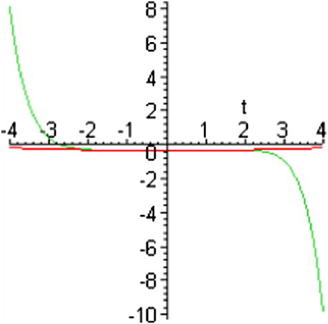
The truncated HPM series solution ψ(x, t) (green) and the exact solution u(x, t) (red) for good Boussinesq equation at c = 0.5 and x = 0.

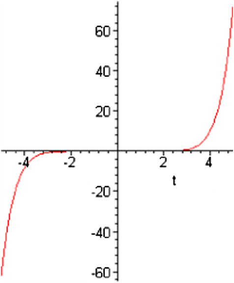
The error between the exact solution u(x, t) and the truncated series solution ψ(x, t) for Boussinesq equation at c = 0.5 and x = 0. We can say that He's semi-inverse method gives exact solution and HPM gives numerical solution from the figures.

4 Conclusion

In this paper, He's semi-inverse method has been tested by applying it successfully to good Boussinesq equation. The most interesting feature of the method is its simplicity coupled with the accuracy. We have also made the comparison of results with He's homotopy perturbation method (HPM). Hence it may be concluded that He's semi-inverse method can be applied to other nonlinear equations arising in mathematical physics and nonlinear sciences.

References

Adomian G., . A review of the decomposition method in applied mathematics. J. Math. Anal. Appl.. 1988;135:501-544.
[Google Scholar]
El-Sayed S.M., . The decomposition method for studying the Klein–Gordon equation. Chaos, Solitons and Fractals. 2003;18(5):1025-1030.
[Google Scholar]
He J.H., . Semi-inverse method of establishing generalized variational principles for fluid mechanics with emphasis on turbo machinery aerodynamics. International Journal of Turbo Jet-Engines. 1997;14(1):23-28.
[Google Scholar]
He J.H., . Variational iteration method – a kind of non-linear analytical technique: some examples. International Journal of Non-linear Mechanics. 1999;34:699-708.
[Google Scholar]
He J.H., . Homotopy perturbation technique. Computer Methods in Applied Mechanics and Engineering. 1999;178(3–4):257-262.
[Google Scholar]
He J.H., . Variational iteration method for autonomous ordinary differential system. Applied Mathematics and Computation. 2000;114:115-123.
[Google Scholar]
He J.H., . Variational principles for some nonlinear partial differential equations with variable coefficients. Chaos, Solitons and Fractals. 2004;19:847-851.
[Google Scholar]
He J.H., . Asymptotology by homotopy perturbation method. Applied Mathematics and Computation. 2004;156(3):591-596.
[Google Scholar]
He J.H., . The homotopy perturbation method for nonlinear oscillators with discontinuities. Applied Mathematics and Computation. 2004;151(1):287-292.
[Google Scholar]
He J.H., . Homotopy perturbation method for bifurcation of nonlinear problems. International Journal of Nonlinear Sciences and Numerical Simulation. 2005;6(2):207-208.
[Google Scholar]
He J.H., . Application of homotopy perturbation method to nonlinear wave equations. Chaos Solitons and Fractals. 2005;26(3):695-700.
[Google Scholar]
He, J.H., 2006. Non-perturbative methods for strongly nonlinear problems. Dissertation de-Verlag im Internet GmbH.
He J.H., . Some asymptotic methods for strongly nonlinear equations. International Journal of Modern Physics B. 2006;20(10):1141-1199.
[Google Scholar]
He J.H., Wu X.H., . Construction of solitary solution and compacton-like solution by variational iteration method. Chaos, Soliton and Fractals. 2006;29:108-113.
[Google Scholar]
He J.H., Wu G.C., Austin F., . The variational iteration method which should be followed. Nonlin. Sci. Lett. A. 2010;1(1):1-30.
[Google Scholar]
Liu H.M., . Generalized variational principles forion acoustic plasma waves by He's semi-inverse method. Chaos, Solitons and Fractals. 2005;23(2):573-576.
[Google Scholar]
Mohyud-Din S.T., Noor M.A., . Homotopy perturbation method for solving partial differential equations. Zeitschrift für Naturforschung A-A Journal of Physical Sciences. 2009;64a:157-170.
[Google Scholar]
Mohyud-Din S.T., Noor M.A., Waheed A., . Exp-function method for generalized travelling solutions of good Boussinesq equations. Journal of Applied Mathematics and Computing Springer. 2008;29:81-94. doi: 10.1007/s12190-008-0183-8
[Google Scholar]
Mohyud-Din, S.T., Noor, M.A., Noor, K.I., 2009. Some relatively new techniques for nonlinear problems. Mathematical Problems in Engineering, Article ID 234849, 25 p. doi: 10.1155/2009/234849.
Noor M.A., Mohyud-Din S.T., Waheed A., . Exp-function method for solving Kuramoto–Sivashinsky and Boussinesq equations. Journal of Applied Mathematics and Computing Springer. 2008;29:1-13. doi: 10.1007/s12190-008-0083-y
[Google Scholar]
Öziş T., Yildirim A., . Traveling wave solution of Korteweg-de Vries equation using He's homotopy perturbation method. International Journal of Nonlinear Science and Numerical Simulation. 2007;8:239-242.
[Google Scholar]
Öziş T., Yildirim A., . Determination of periodic solution for a u(1/3) force by He’ s modified Lindstedt–Poincaré method. Journal of Sound and Vibration. 2007;301:415-419.
[Google Scholar]
Öziş T., Yildirim A., . A study of nonlinear oscillators with u^1/3 force by He's variational iteration method. Journal of Sound and Vibration. 2007;306:372-376.
[Google Scholar]
Öziş T., Yıldırım A., . An application of He's semi-inverse method to the nonlinear Schrödinger (NLS) equation. Computer Mathematics with Applications. 2007;54:1039-1042.
[Google Scholar]
Öziş T., Yildirim A., . A note on He's homotopy perturbation method for van der Pol oscillator with very strong nonlinearity. Chaos, Solitons and Fractals. 2007;34:989-991.
[Google Scholar]
Öziş T., Yildirim A., . A comparative study of He's homotopy perturbation method for determining frequency-amplitude relation of a nonlinear oscillator with discontinuities. International Journal of Nonlinear Science and Numerical Simulation. 2007;8:243-248.
[Google Scholar]
Tao, Z.L., in press. Variational approach to the Benjamin Ono equation. Nonlinear Analysis: Real World Applications.
Wazwaz A.M., . A reliable modification of Adomian's decomposition method. Appl. Math. Comput.. 1988;92:1-7.
[Google Scholar]
Wazwaz A.M., . The variational iteration method: a powerful scheme for handling linear and nonlinear diffusion equations. Computer Mathematics with applications. 2007;54:933-939.
[Google Scholar]
Yildirim, A., Öziş, T., in press. Solutions of singular IVPs of Lane–Emden type by the variational iteration method. Nonlinear Analysis: Theory Method Applications.
Yildirim A., Öziş T., . Solutions of singular IVPs of Lane–Emden type by homotopy perturbation method. Physics Letters A. 2007;369:70-76.
[Google Scholar]

Introduction

He's semi-inverse method

Applying homotopy prturbation method (HPM) on good Boussinesq equation

Conclusion

Fulltext Views
28

PDF downloads
2

View/Download PDF
Download Citations

BibTeX
RIS

Show Sections

[1] Adomian G., . A review of the decomposition method in applied mathematics. J. Math. Anal. Appl.. 1988;135:501-544.
[Google Scholar]

[2] El-Sayed S.M., . The decomposition method for studying the Klein–Gordon equation. Chaos, Solitons and Fractals. 2003;18(5):1025-1030.
[Google Scholar]

[3] He J.H., . Semi-inverse method of establishing generalized variational principles for fluid mechanics with emphasis on turbo machinery aerodynamics. International Journal of Turbo Jet-Engines. 1997;14(1):23-28.
[Google Scholar]

[4] He J.H., . Variational iteration method – a kind of non-linear analytical technique: some examples. International Journal of Non-linear Mechanics. 1999;34:699-708.
[Google Scholar]

[5] He J.H., . Homotopy perturbation technique. Computer Methods in Applied Mechanics and Engineering. 1999;178(3–4):257-262.
[Google Scholar]

[6] He J.H., . Variational iteration method for autonomous ordinary differential system. Applied Mathematics and Computation. 2000;114:115-123.
[Google Scholar]

[7] He J.H., . Variational principles for some nonlinear partial differential equations with variable coefficients. Chaos, Solitons and Fractals. 2004;19:847-851.
[Google Scholar]

[8] He J.H., . Asymptotology by homotopy perturbation method. Applied Mathematics and Computation. 2004;156(3):591-596.
[Google Scholar]

[9] He J.H., . The homotopy perturbation method for nonlinear oscillators with discontinuities. Applied Mathematics and Computation. 2004;151(1):287-292.
[Google Scholar]

[10] He J.H., . Homotopy perturbation method for bifurcation of nonlinear problems. International Journal of Nonlinear Sciences and Numerical Simulation. 2005;6(2):207-208.
[Google Scholar]

[11] He J.H., . Application of homotopy perturbation method to nonlinear wave equations. Chaos Solitons and Fractals. 2005;26(3):695-700.
[Google Scholar]

[12] He, J.H., 2006. Non-perturbative methods for strongly nonlinear problems. Dissertation de-Verlag im Internet GmbH.

[13] He J.H., . Some asymptotic methods for strongly nonlinear equations. International Journal of Modern Physics B. 2006;20(10):1141-1199.
[Google Scholar]

[14] He J.H., Wu X.H., . Construction of solitary solution and compacton-like solution by variational iteration method. Chaos, Soliton and Fractals. 2006;29:108-113.
[Google Scholar]

[15] He J.H., Wu G.C., Austin F., . The variational iteration method which should be followed. Nonlin. Sci. Lett. A. 2010;1(1):1-30.
[Google Scholar]

[16] Liu H.M., . Generalized variational principles forion acoustic plasma waves by He's semi-inverse method. Chaos, Solitons and Fractals. 2005;23(2):573-576.
[Google Scholar]

[17] Mohyud-Din S.T., Noor M.A., . Homotopy perturbation method for solving partial differential equations. Zeitschrift für Naturforschung A-A Journal of Physical Sciences. 2009;64a:157-170.
[Google Scholar]

[18] Mohyud-Din S.T., Noor M.A., Waheed A., . Exp-function method for generalized travelling solutions of good Boussinesq equations. Journal of Applied Mathematics and Computing Springer. 2008;29:81-94. doi: 10.1007/s12190-008-0183-8
[Google Scholar]

[19] Mohyud-Din, S.T., Noor, M.A., Noor, K.I., 2009. Some relatively new techniques for nonlinear problems. Mathematical Problems in Engineering, Article ID 234849, 25 p. doi: 10.1155/2009/234849.

[20] Noor M.A., Mohyud-Din S.T., Waheed A., . Exp-function method for solving Kuramoto–Sivashinsky and Boussinesq equations. Journal of Applied Mathematics and Computing Springer. 2008;29:1-13. doi: 10.1007/s12190-008-0083-y
[Google Scholar]

[21] Öziş T., Yildirim A., . Traveling wave solution of Korteweg-de Vries equation using He's homotopy perturbation method. International Journal of Nonlinear Science and Numerical Simulation. 2007;8:239-242.
[Google Scholar]

[22] Öziş T., Yildirim A., . Determination of periodic solution for a u(1/3) force by He’ s modified Lindstedt–Poincaré method. Journal of Sound and Vibration. 2007;301:415-419.
[Google Scholar]

[23] Öziş T., Yildirim A., . A study of nonlinear oscillators with u^1/3 force by He's variational iteration method. Journal of Sound and Vibration. 2007;306:372-376.
[Google Scholar]

[24] Öziş T., Yıldırım A., . An application of He's semi-inverse method to the nonlinear Schrödinger (NLS) equation. Computer Mathematics with Applications. 2007;54:1039-1042.
[Google Scholar]

[25] Öziş T., Yildirim A., . A note on He's homotopy perturbation method for van der Pol oscillator with very strong nonlinearity. Chaos, Solitons and Fractals. 2007;34:989-991.
[Google Scholar]

[26] Öziş T., Yildirim A., . A comparative study of He's homotopy perturbation method for determining frequency-amplitude relation of a nonlinear oscillator with discontinuities. International Journal of Nonlinear Science and Numerical Simulation. 2007;8:243-248.
[Google Scholar]

[27] Tao, Z.L., in press. Variational approach to the Benjamin Ono equation. Nonlinear Analysis: Real World Applications.

[28] Wazwaz A.M., . A reliable modification of Adomian's decomposition method. Appl. Math. Comput.. 1988;92:1-7.
[Google Scholar]

[29] Wazwaz A.M., . The variational iteration method: a powerful scheme for handling linear and nonlinear diffusion equations. Computer Mathematics with applications. 2007;54:933-939.
[Google Scholar]

[30] Yildirim, A., Öziş, T., in press. Solutions of singular IVPs of Lane–Emden type by the variational iteration method. Nonlinear Analysis: Theory Method Applications.

[31] Yildirim A., Öziş T., . Solutions of singular IVPs of Lane–Emden type by homotopy perturbation method. Physics Letters A. 2007;369:70-76.
[Google Scholar]