A single server Non-Markovian with non-compulsory re-service and balking under Modified Bernoulli Vacation

Bharathi J.; Nandhini S.

doi:10.1016/j.jksus.2023.103007

View/Download PDF

Buy Reprints

PDF

Translate this page into:

01 2023

:36;

103007

doi:

10.1016/j.jksus.2023.103007

A single server Non-Markovian with non-compulsory re-service and balking under Modified Bernoulli Vacation

Bharathi J., Nandhini S.^⁎

Department of Mathematics, School of Advanced Sciences, Vellore Institute of Technology, Vellore, Tamilnadu, India

⁎Corresponding author. nandhini.s@vit.ac.in (Nandhini S.)

Received: 2022-9-21, Accepted: 2023-11-10,

Disclaimer:
This article was originally published by Elsevier and was migrated to Scientific Scholar after the change of Publisher.

Abstract

In this paper, a single-server queue with Modified Bernoulli Vacation(MBV) has been considered. The server provides two kinds of services, Compulsory Service (CR) and Non-Compulsory Re-service (NCR). Any new customer who arrives and finds the server engaged, on breakdown, or on vacation will be placed on an orbit; or else if he finds the server free, he enters the service immediately. The server takes a vacation as soon as the orbit is empty at the usual service completion moment. The dissatisfied customer may re-enter the orbit after usual service is complete to receive another service. We have used SVM (Supplementary Variable Method) to derive PGF (Probability Generating Function) for the system. In order to demonstrate the influence that the system parameters have, numerical examples are discussed.

Keywords

Retry queues

Non-compulsory re-service

Modified Bernoulli vacation

Breakdown

Show Related Articles from PubMed

1 Introduction

Retrial queuing is a queueing paradigm in which a randomly arriving customer observes that the server is busy and starts to make repetitive client requests called as orbit. An impatient customer is one who enters the queue in a reneging or balking state, becomes impatient rapidly, and may depart the system before the service is completed. In this work, we have derived the steady state equations for the case of impatient customers in retrial queuing model and derived some significant performance metrics of the model.

The review of the literature on retry queue can be found in Falin and Templeton (1997). In Gomez-Corral (1999) a Non-Markovian queueing system with generic retrial times has been analyzed. A two phase service pattern with retrial queuing has been presented in Artalejo and Choudhury (2004). Phases 1 and 2 of the service are taken into consideration, and significant performance metrics are derived. Under the Bernoulli schedule, a single-server queue with phase1 and phase2 service and a MBV is discussed in Jain and Agarwal (2010). A hybrid queueing model with weighted fair queueing and differential packet dropping is used in congestion control in networks (Nandhini, 2013). In a recent study in Ke et al. (2010), a wide range of vacation rules were examined. Doshi (1986) has discussed significant concepts on single-server queues with vacations. An $M / G / 1$ retrial queue in which the customer chooses for second phase multi-optional service (SMOS) has been discussed in Wang and Li (2009). In Madheswari et al. (2019), the authors have investigated a single server retrial queue of two phases of service that operates under the Bernoulli vacation in which they consider the second phase as optional. Retrial queue with two phases of service, balking, vacations (Bernoulli and Modified Bernoulli), feedback has been investigated in Arivudainambi and Godhandaraman (2012), Choudhury and Madan (2005), Choudhury and Deka (2008).

The retrying client has a significant impact on the dynamics of coupled switching in ATM centers, which is an extremely important factor to consider. The intervals between subsequent retrials, however, rely less on the quantity of customers who have attempted it in a certain service settings. In these circumstances, it is assumed that only the customer who is at the head of the orbit is permitted for retrial service, as in Dimitriou (2018), or alternatively, after a service has been provided, the server may seek customers from the orbit. The authors of a recent study in Legros (2021, 2022) examined the admission control problem with state-dependent arrivals and proposed a system sizing algorithm and has shown that the wait time can be reduced by taking use of the latest recent event. There have also been other single-server queueing models proposed in Boxma and Vlasiou (2007), Kerner (2008) where the arrival or service rates depend on the customer’s wait time while getting service or standing in the queue.

Analysis has been carried out on an SSMQS (single server Markovian queueing system) (Bouchentouf et al., 2021), which included balking, Bernoulli feedback and its server states dependent on reneging, as well as retention of reneged consumers under a variation multiple policies (vacation). In Boussaha et al. (2022), study has been performed on a single server feedback retrial queueing system (SSFRQM) using orbital search customers. Balking consumers, UDRQ (Uncertain Discrete-time Retrial Queue) with PPP (Probabilistic Preemptive Priority)and RRT (Replacements of Repair Times) were recently examined in Lan and Tang (2020).

Retrial models appear naturally in HMS (Healthcare Management System), WSN (Wireless Sensor Network), CTN (Communication and Transportation Networks), IOT (Internet of Things), TS (Task Scheduling), TE (Traffic Engineering), TCC (Telecommunication and Call Centre) and ICS (Inventory Control System).

Retrial queueing model with Bernoulli vacation is our primary focus of interest. Past literatures were dealing with a Single-Server Retrial Queue Model (SSRQM), with two stages of service and Bernoulli vacation. This paper presents an advanced SSRQM which comprises of two phases of services (CR and NCR) under Modified Bernoulli Vacation (MBV) added with balking state also. The uniqueness of our approach also includes the consideration of repair and breakdown under MBV. Prominent performance measures has been derived for our model and numerical analysis and graphical representation of the model has also been presented.

The structure of this paper is structured as follows. In Section 2, we present the mathematical description of the system under consideration. In Section 3 steady state equations and PGF of system size, orbit size are presented. Several system performance measures are discussed in Section 4. The special cases of the proposed model is covered in Section 5. Numerical Illustrations are discussed in Section 6 and Section 7 conclusion and future work is presented.

2 Mathematical description

The service discipline for new arriving customers is FIFO. We assume a single Poisson arrival with $λ$ as the mean rate. The retrial-service is generally distributed with its distribution function $ϖ (ħ_{l})$ , df(density function) $κ (ħ_{l})$ , and LST (Laplace–Stieltjes transform) $ϖ^{*} (ħ_{l})$ . The service time distribution function $U_{1} (ȷ_{q})$ for compulsory service and $U_{2} (ȷ_{q})$ for non-compulsory (re-service), LST $U_{1}^{*} (ħ_{l}), U_{2}^{*} (ħ_{l})$ , its first two moments are $\bar{\bar{\dot{S_{i}^{1}}}}$ and $\bar{\bar{\dot{S_{i}^{2}}}}$ respectively $i = 1, 2$ . After completion of each service, the server takes MBV, with its distribution function $B (ȷ_{q})$ and LST $B^{*} (ħ_{l})$ its first two moments ${\bar{\bar{v}}}^{(1)}$ , ${\bar{\bar{v}}}^{(2)}$ .

An entering customer is served by a single server on a FIFO basis. When the service is finished, some of the approaching customers may opt to NCR with probability $r_{1}$ or depart with probability $\bar{r_{1}} = 1 - r_{1}$ . Balking may occur whenever a customer enters the service area with a probability $1 - \bar{\bar{b}}$ and the customer exits with probability $\bar{\bar{b}}$ . The server waits with probability $1 - c$ and goes on vacation with probability $c$ if no customers are present at the end of each service.

Both the services, vacation, delay time and repair time follows general distribution.

Let $I (ȷ_{q}) = \{\begin{matrix} 0 & \to server is inactive \\ 1 & \to server is engaged \\ 2 & \to server is on non-compulsory re-service \\ 3 & \to server is delaying repair on compulsory service \\ 4 & \to server is delaying repair on non-compulsory re-service \\ 5 & \to server is repair on compulsory service \\ 6 & \to server is repair on non-compulsory re-service \\ 7 & \to server is on vacation \end{matrix}$

We assume that breakdown of the server for both the services are according to Poisson stream with mean breakdown rates $γ_{1}$ and $γ_{2}$ . The delay time distribution function $W_{i} (ȷ_{q})$ and LST $W_{i}^{*} (ħ_{m})$ , respectively and its moments are $\bar{\bar{\dot{g_{i}^{1}}}}$ , $\bar{\bar{\dot{g_{i}^{2}}}}$ , $i = 1, 2$ , and the repair time of distribution function are $E_{i} (ȷ_{q})$ and LST $E_{i}^{*} (ħ_{m})$ , respectively and its moments are $\bar{\bar{\dot{f_{i}^{1}}}}$ , $\bar{\bar{\dot{f_{i}^{2}}}}$ .

Let us assume $ϖ (0) = 0, ϖ (\infty) = 1, U_{1} (0) = 0, U_{1} (\infty) = 1, U_{2} (0) = 0, U_{2} (\infty) = 1, B (0) = 0, B (\infty) = 1$ are continuous at $ħ_{l} = 0$ and $W_{i} (0) = 0, W_{i} (\infty) = 1, E_{i} (0) = 0, E_{i} (\infty) = 1$ are continuous at $ħ_{m} = 0$ .

Hazard rates of the conditions(retrial, services,vacation, repairs) are $κ (ħ_{l}) d ħ_{l} = \frac{d ϖ (ħ_{l})}{1 - ϖ (ħ_{l})} (repeated attempts)$ $η_{1} (ħ_{l}) d ħ_{l} = \frac{d U_{1} (ħ_{l})}{1 - U_{1} (ħ_{l})} (compulsory service)$ $η_{2} (ħ_{l}) d ħ_{l} = \frac{d U_{2} (ħ_{l})}{1 - U_{2} (ħ_{l})} (non-compulsory re-service)$ $ν (ħ_{l}) d ħ_{l} = \frac{d B (ħ_{l})}{1 - B (ħ_{l})} (vacation)$ $β_{i} (ħ_{m}) d ħ_{m} = \frac{d W_{i} (ħ_{m})}{1 - W_{j} (ħ_{m})}, i = 1, 2 (delaying repair on both services)$ $ω_{i} (ħ_{m}) d ħ_{m} = \frac{d E_{i} (ħ_{m})}{1 - E_{i} (ħ_{m})}, i = 1, 2 (repair on both services)$

3 Steady state formulation and solution

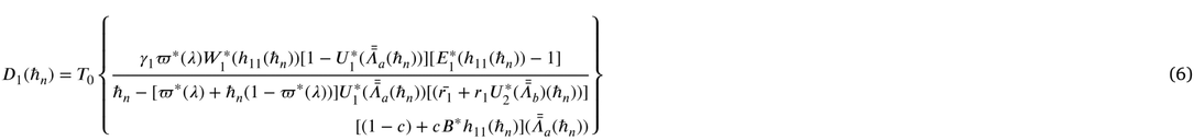
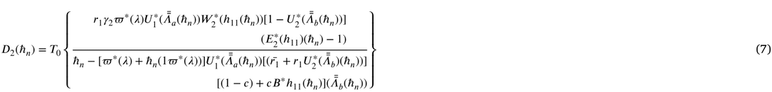
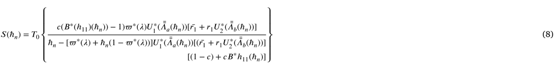
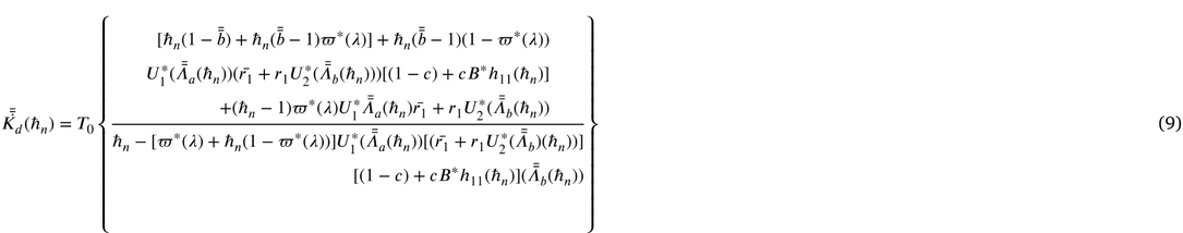
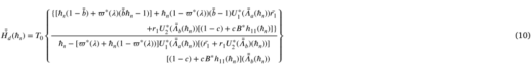
In this section, we have presented the steady-state through Eqs. (1) to (16), and the boundary conditions are given in Eqs. (17) through (25). Applying PGF we arrive Eqs. (27) to (42). Finally, we have presented the probability generating function of orbit size while the server is idle, busy on CR or NCR, on MBV, under postponing repair on CR or NCR, and repair on CR or NCR accordingly.

Notations used

$T_{0} (ȷ_{q})$ $\to$ The prob(probability) that the system is idle at $ȷ_{q}$ .

$T_{ı_{p}} (ħ_{l}, ȷ_{q})$ $\to$ The prob that at $ȷ_{q}$ there are precisely $ı_{p}$ customers in the orbit with elapsed time (retrial) $ħ_{l}$ ,of customers going-through retrial .

$φ_{(1, ı_{p})} (ħ_{l}, ȷ_{q})$ $\to$ The prob that at $ȷ_{q}$ there are precisely $ı_{p}$ customers in orbit with elapsed time (CR) of the customer $ħ_{l}$ going-through service .

$φ_{(2, ı_{p})} (ħ_{l}, ȷ_{q})$ $\to$ The prob that at $ȷ_{q}$ there are precisely $ı_{p}$ customers in the orbit with elapsed time (re-service) on NCR of the customer $ħ_{l}$ going-through service .

$Q_{(1, ı_{p})} (ħ_{l}, ħ_{m}, ȷ_{q})$ $\to$ The prob that at $ȷ_{q}$ there are precisely $ı_{p}$ customers in orbit with the elapsed time (CR) of test customer $ħ_{l}$ going-through service and the elapsed (delaying repair) of server is $ħ_{m}$ .

$Q_{(2, ı_{p})} (ħ_{l}, ħ_{m}, ȷ_{q})$ $\to$ The prob that at $ȷ_{q}$ there are precisely $ı_{p}$ customers in the orbit with elapsed time NCR of the customers going-through service is $ħ_{l}$ and the elapsed (delaying repair) of server is $ħ_{m}$ .

$D_{(1, ı_{p})} (ħ_{l}, ħ_{m}, ȷ_{q})$ $\to$ The prob that at $ȷ_{q}$ there are precisely $ı_{p}$ customers in orbit with elapsed time (CR) time of the customers going-through service is $ħ_{l}$ and the elapsed (repair) time of server is $ħ_{m}$ .

$D_{(2, ı_{p})} (ħ_{l}, ħ_{m}, ȷ_{q})$ $\to$ The prob that at $ȷ_{q}$ there are precisely $ı_{p}$ customers in the orbit with the elapsed time (NCR) of the test customer going-through service is $ħ_{l}$ and the elapsed (repair) time of server is $ħ_{m}$ .

$S_{ı_{p}} (ħ_{l}, ȷ_{q})$ $\to$ The prob that at $ȷ_{q}$ there are precisely $ı_{p}$ customers in orbit with elapsed (vacation) time $ħ_{l}$ .

The probabilities are described as: $T_{0} (ȷ_{q}) = T {I (ȷ_{q}) = 0, \bar{\bar{\dot{X}}} (ȷ_{q}) = 0}$ $T_{ı_{p}} (ħ_{l}, ȷ_{q}) d ħ_{l} = P {I (ȷ_{q}) = 0, \bar{\bar{\dot{X}}} (ȷ_{q}) = ı_{p}, ħ_{l} \leq ϖ^{0} (ȷ_{q}) < ħ_{l} + d ħ_{l}}, ı_{p} \geq 1$ $φ_{(1, ı_{p})} (ħ_{l}, ȷ_{q}) d ħ_{l} = P {I (ȷ_{q}) = 1, \bar{\bar{\dot{X}}} (ȷ_{q}) = ı_{p}, ħ_{l} \leq U_{1}^{0} (t) < ħ_{l} + d ħ_{l}} for ȷ_{q}, ħ_{l}, ı_{p} \geq 0$ $φ_{(2, ı_{p})} (ħ_{l}, ȷ_{q}) d ħ_{l} = P {I (ȷ_{q}) = 2, \bar{\bar{\dot{X}}} (ȷ_{q}) = ı_{p}, ħ_{l} \leq U_{2}^{0} (t) < ħ_{l} + d ħ_{l}}$ $Q_{(1, ı_{p})} (ħ_{l}, ħ_{m}, ȷ_{q}) d ħ_{m} = P {I (ȷ_{q}) = 3, \bar{\bar{\dot{X}}} (ȷ_{q}) = ı_{p}, ħ_{m} \leq W_{1}^{0} (ȷ_{q}) < ħ_{m} + d ħ_{m} / U_{1}^{0} (ȷ_{q}) = ȷ_{q}} for ȷ_{q}, ħ_{l}, ı_{p} \geq 0$ $Q_{(2, ı_{p})} (ħ_{l}, ħ_{m}, ȷ_{q}) d ħ_{m} = P {I (ȷ_{q}) = 4, \bar{\bar{\dot{X}}} (ȷ_{q}) = ı_{p}, ħ_{m} \leq W_{2}^{0} (ȷ_{q}) < ħ_{m} + d ħ_{m} / U_{2}^{0} (ȷ_{q}) = ħ_{l}}$ $D_{(1, ı_{p})} (ħ_{l}, ħ_{m}, ȷ_{q}) d ħ_{m} = P {I (ȷ_{q}) = 5, \bar{\bar{\dot{X}}} (ȷ_{q}) = ı_{p}, ħ_{m} \leq E_{1}^{0} (ȷ_{q}) < ħ_{m} + d ħ_{m} / U_{1}^{0} (ȷ_{q}) = ħ_{l}} for ȷ_{q}, ħ_{l}, ı_{p} \geq 0$ $D_{(2, ı_{p})} (ħ_{l}, ħ_{m}, ȷ_{q}) d ħ_{m} = P {I (ȷ_{q}) = 6, \bar{\bar{\dot{X}}} (ȷ_{q}) = ı_{p}, ħ_{m} \leq E_{2}^{0} (\bar{\bar{\dot{t_{1}}}}) < ħ_{m} + d ħ_{m} / U_{2}^{0} (\bar{\bar{\dot{t_{1}}}}) = ħ_{l}}$ $S_{ı_{p}} (ħ_{l}, ȷ_{q}) d ħ_{l} = P {I (ȷ_{q}) = 7, \bar{\bar{\dot{X}}} (ȷ_{q}) = ı_{p}, ħ_{l} \leq B^{0} (ȷ_{q}) < ħ_{l} + d ħ_{l}}$

The set of governing equations (behavior of dynamic system) are given by

(1)

λ \bar{\bar{b}} T_{0} = (1 - c) [\bar{r_{1}} \int_{0}^{\infty} φ_{(1, 0)} (ħ_{l}) η_{1} (ħ_{l}) d ħ_{l} + \int_{0}^{\infty} φ_{(2, 0)} (ħ_{l}) η_{2} (ħ_{l}) d ħ_{l}]

+ \int_{0}^{\infty} S_{0} (ħ_{l}) ν (ħ_{l}) d ħ_{l}

(2)

\frac{d T_{ı_{p}} (ħ_{l})}{d ħ_{l}} + (λ + κ (ħ_{l})) T_{ı_{p}} (ħ_{l}) = 0

(3)

\frac{d φ_{1, 0} (ħ_{l})}{d ħ_{l}} + [\bar{\bar{b}} λ + γ_{1} + η_{1} (ħ_{l})] φ_{1, 0} (ħ_{l}) = \int_{0}^{\infty} β_{1} (ħ_{m}) Q_{1, 0} (ħ_{l}, ħ_{m}) d ħ_{m}

(4)

\frac{d φ_{1, ı_{p}} (ħ_{l})}{d ħ_{l}} + [\bar{\bar{b}} λ + γ_{1} + η_{1} (ħ_{l})] φ_{1, ı_{p}} (ħ_{l}) = \bar{\bar{b}} λ φ_{1, ı_{p} - 1} (ħ_{l}) + \int_{0}^{\infty} β_{1} (ħ_{m}) Q_{1, ı_{p}} (ħ_{l}, ħ_{m}) d ħ_{m}, ı_{p} \geq 1

(5)

\frac{d φ_{2, 0} (ħ_{l})}{d ħ_{l}} + [\bar{\bar{b}} λ + γ_{2} + η_{2} (ħ_{l})] φ_{2, 0} (ħ_{l}) = \int_{0}^{\infty} β_{2} (ħ_{m}) Q_{2, 0} (ħ_{l}, ħ_{m}) d ħ_{m}

(6)

\frac{d φ_{2, ı_{p}} (ħ_{l})}{d ħ_{l}} + [\bar{\bar{b}} λ + γ_{2} + η_{2} (ħ_{l})] φ_{2, ı_{p}} (ħ_{l}) = \bar{\bar{b}} λ φ_{2, ı_{p} - 1} (ħ_{l}) + \int_{0}^{\infty} β_{2} (ħ_{m}) Q_{2, ı_{p}} (ħ_{l}, ħ_{m}) d ħ_{m}, ı_{p} \geq 1

(7)

\frac{d Q_{1, 0} (ħ_{l}, ħ_{m})}{d ħ_{m}} + (\bar{\bar{b}} λ + β_{1} (ħ_{m})) Q_{1, 0} (ħ_{l}, ȷ_{q}) = 0

(8)

\frac{d Q_{1, ı_{p}} (ħ_{l}, ħ_{m})}{d ħ_{m}} + (\bar{\bar{b}} λ + β_{1} (ħ_{m})) Q_{1, ı_{p}} (ħ_{l}, ħ_{m}) = \bar{\bar{b}} λ Q_{1, ı_{p} - 1} (ħ_{l}, ħ_{m}), ı_{p} \geq 1

(9)

\frac{d Q_{2, 0} (ħ_{l}, ħ_{m})}{d ħ_{m}} + (\bar{\bar{b}} λ + β_{2} (ħ_{m})) Q_{2, 0} (ħ_{l}, ħ_{m}) = 0

(10)

\frac{d Q_{2, ı_{p}} (ħ_{l}, ħ_{m})}{d ħ_{m}} + (\bar{\bar{b}} λ + β_{2} (ħ_{m})) Q_{2, ı_{p}} (ħ_{l}, ħ_{m}) = \bar{\bar{b}} λ Q_{2, ı_{p} - 1} (ħ_{l}, ħ_{m}), ı_{p} \geq 1

(11)

\frac{d D_{1, 0} (ħ_{l}, ħ_{m})}{d ħ_{m}} + (\bar{\bar{b}} λ + ω_{1} (ħ_{m})) D_{1, 0} (ħ_{l}, ħ_{m}) = 0

(12)

\frac{d D_{1, ı_{p}} (ħ_{l}, ħ_{m})}{d ħ_{m}} + (\bar{\bar{b}} λ + ω_{1} (ħ_{m})) D_{1, ı_{p}} (ħ_{l}, ħ_{m}) = \bar{\bar{b}} λ D_{1, ı_{p} - 1} (ħ_{l}, ħ_{m}), ı_{p} \geq 1

(13)

\frac{d D_{2, 0} (ħ_{l}, ħ_{m})}{d ħ_{m}} + (\bar{\bar{b}} λ + ω_{2} (ħ_{m})) D_{2, 0} (ħ_{l}, ħ_{m}) = 0

(14)

\frac{d D_{2, ı_{p}} (ħ_{l}, ħ_{m})}{d ħ_{m}} + (\bar{\bar{b}} λ + ω_{2} (ħ_{m})) D_{2, ı_{p}} (ħ_{l}, ħ_{m}) = \bar{\bar{b}} λ D_{2, ı_{p} - 1} (ħ_{l}, ħ_{m}), ı_{p} \geq 1

(15)

\frac{d S_{0} (ħ_{l})}{d ħ_{l}} + (\bar{\bar{b}} λ + ν (ħ_{l})) S_{0} (ħ_{l}) = 0

(16)

\frac{d S_{ı_{p}} (ħ_{l})}{d ħ_{l}} + (\bar{\bar{b}} λ + ν (ħ_{l}) S_{ı_{p}} (ħ_{l}) = \bar{\bar{b}} λ S_{ı_{p} - 1} (ħ_{l})), ı_{p} \geq 1

The following boundary conditions (

ħ_{l} = 0, ħ_{m} = 0

) are used to solve the set of Eqs. (1) to (16).

(17)

T_{ı_{p}} (0) = (1 - c) [\bar{r_{1}} \int_{0}^{\infty} φ_{(1, ı_{p})} (ħ_{l}) η_{1} (ħ_{l}) d ħ_{l} + \int_{0}^{\infty} φ_{(2, ı_{p})} (ħ_{l}) η_{2} (ħ_{l}) d ħ_{l}]

+ \int_{0}^{\infty} S_{ı_{p}} (ħ_{l}) ν (ħ_{l}) d ħ_{l}

(18)

φ_{1, ı_{p}} (0) = \int_{0}^{\infty} T_{1} (ħ_{l}) κ (ħ_{l}) d ħ_{l} + \bar{\bar{b}} λ T_{0}

(19)

φ_{1, ı_{p}} (ħ_{l}, 0) = \int_{0}^{\infty} T_{ı_{p} + 1} (ħ_{l}) κ (ħ_{l}) d ħ_{l} + λ \int_{0}^{\infty} T_{ı_{p}} (ħ_{l}) d ħ_{l}

(20)

φ_{2, ı_{p}} (ħ_{l}, 0) = β_{1} \int_{0}^{\infty} φ_{1, ı_{p}} (ħ_{l}) η_{1} (ħ_{l}) d ħ_{l}

(21)

Q_{1, ı_{p}} (ħ_{l}, 0) = γ_{1} φ_{1, ı_{p}} (ħ_{l})

(22)

Q_{2, ı_{p}} (ħ_{l}, 0) = γ_{2} φ_{2, ı_{p}} (ħ_{l})

(23)

D_{1, ı_{p}} (ħ_{l}, 0) = \int_{0}^{\infty} Q_{1, ı_{p}} β_{1} (ħ_{m}) d ħ_{m}

(24)

D_{2, ı_{p}} (ħ_{l}, 0) = \int_{0}^{\infty} Q_{2, ı_{p}} β_{2} (ħ_{m}) d ħ_{m}

(25)

S_{ı_{p}} (0) = c \bar{r_{1}} \int_{0}^{\infty} φ_{1, ı_{p}} (ħ_{l}) η_{1} (ħ_{l}) d ħ_{l} + c \int_{0}^{\infty} φ_{2, ı_{p}} (ħ_{l}) η_{2} (ħ_{l}) d ħ_{l}, ı_{p} \geq 1

The normalizing condition is given by

(26)

T_{0} + \sum_{ı_{p} = 1}^{\infty} \int_{0}^{\infty} T_{ħ_{l}} (ħ_{l}) d ħ_{l} + \sum_{ı_{p} = 0}^{\infty} [\int_{0}^{\infty} φ_{1, ı_{p}} (ħ_{l}) d ħ_{l} + \int_{0}^{\infty} φ_{2, ı_{p}} (ħ_{l}) d ħ_{l}

+ \int_{0}^{\infty} S_{ı_{p}} (ħ_{l}) d ħ_{l} + \int_{0}^{\infty} \int_{0}^{\infty} Q_{1, ı_{p}} (ħ_{l}, ħ_{m}) d ħ_{l} d ħ_{m}

+ \int_{0}^{\infty} \int_{0}^{\infty} Q_{2, ı_{p}} (ħ_{l}, ħ_{m}) d ħ_{l} d ħ_{m}

+ \int_{0}^{\infty} \int_{0}^{\infty} D_{1, ı_{p}} (ħ_{l}, ħ_{m}) d ħ_{l} d ħ_{m} + \int_{0}^{\infty} \int_{0}^{\infty} D_{2, ı_{p}} (ħ_{l}, ħ_{m}) d ħ_{l} d ħ_{m}] = 1

The probability generating functions would be defined as follows:

T (ħ_{l}, ħ_{n}) = \sum_{ı_{p} = 0}^{\infty} T_{ı_{p}} (ħ_{l}) {ħ_{n}}^{ı_{p}} for ħ_{l} > 0, T (0, ħ_{n}) = \sum_{ı_{p} = 0}^{\infty} T_{ı_{p}} (0) {ħ_{n}}^{ı_{p}}

φ_{i} (ħ_{l}, ħ_{n}) = \sum_{ı_{p} = 0}^{\infty} φ_{i, ı_{p}} (ħ_{l}) {ħ_{n}}^{ı_{p}}, φ_{i} (0, ħ_{n}) = \sum_{ı_{p} = 0}^{\infty} φ_{i} ı_{p} (0) {ħ_{n}}^{ı_{p}}

Q_{i} (ħ_{l}, ħ_{m}, ħ_{n}) = \sum_{ı_{p} = 0}^{\infty} Q_{i, ı_{p}} (ħ_{l}, ħ_{m}) {ħ_{n}}^{ı_{p}}, Q_{i} (ħ_{l}, 0, ħ_{n}) = \sum_{ı_{p} = 0}^{\infty} Q_{i} ı_{p} (ħ_{l}, 0) {ħ_{n}}^{ı_{p}}

D_{i} (ħ_{l}, ħ_{m}, ħ_{n}) = \sum_{ı_{p} = 0}^{\infty} D_{i, ı_{p}} (ħ_{l}, ħ_{m}) {ħ_{n}}^{ı_{p}}, D_{i} (ħ_{l}, 0, ħ_{n}) = \sum_{ı_{p} = 0}^{\infty} D_{i} ı_{p} (ħ_{l}, 0) {ħ_{n}}^{ı_{p}}

S_{ı_{p}} (ħ_{l}) {ħ_{n}}^{ı_{p}} for ħ_{l} > 0, S (0, ħ_{n}) = \sum_{ı_{p} = 0}^{\infty} S_{ı_{p}} (0) {ħ_{n}}^{ı_{p}}

Now multiply Eq. (2) to (25) by $ħ_{n}$ and adding up all the values of $ı_{p}$ (summing), we obtain

(27)

\frac{d T (ħ_{l}, ħ_{n})}{d ħ_{l}} + (λ + κ (ħ_{l})) T (ħ_{l}, ħ_{n}) = 0

(28)

\frac{d φ_{1} (ħ_{l}, ħ_{n})}{ħ_{l}} + [\bar{\bar{b}} λ (1 - ħ_{n}) + γ_{1} + η_{1} (ħ_{l})] φ_{1} (ħ_{l}, ħ_{n}) = \int_{0}^{\infty} β_{1} (ħ_{m}) Q_{1} (ħ_{l}, ħ_{m}, ħ_{n}) d ħ_{m}

(29)

\frac{d φ_{2} (ħ_{l}, ħ_{n})}{d ħ_{l}} + [\bar{\bar{b}} λ (1 - ħ_{n}) + γ_{2} + η_{2} (ħ_{l})] φ_{2} (ħ_{l}, ħ_{n}) = \int_{0}^{\infty} β_{2} (ħ_{m}) Q_{2} (ħ_{l}, ħ_{m}, ħ_{n}) d ħ_{m}

(30)

\frac{d Q_{1} (ħ_{l}, ħ_{m}, ħ_{n})}{ħ_{m}} + (\bar{\bar{b}} λ (1 - ħ_{n}) + β_{1} (ħ_{m})) Q_{1} (ħ_{l}, ħ_{m}, ħ_{n}) = 0

(31)

\frac{d Q_{2} (ħ_{l}, ħ_{m}, ħ_{n})}{ħ_{m}} + (\bar{\bar{b}} λ (1 - ħ_{n}) + β_{2} (ħ_{m})) Q_{2} (ħ_{l}, ħ_{m}, ħ_{n}) = 0

(32)

\frac{d D_{1} (ħ_{l}, ħ_{m}, ħ_{n})}{d ħ_{m}} + (\bar{\bar{b}} λ (1 - ħ_{n}) + ω_{1} (ħ_{m})) Q_{1} (ħ_{l}, ħ_{m}, ħ_{n}) = 0

(33)

\frac{d D_{2} (ħ_{l}, ħ_{m}, ħ_{n})}{d ħ_{m}} + (\bar{\bar{b}} λ (1 - ħ_{n}) + ω_{2} (ħ_{m})) Q_{2} (ħ_{l}, ħ_{m}, ħ_{n}) = 0

(34)

\frac{d S (ħ_{l}, ħ_{n})}{d ħ_{l}} + (\bar{\bar{b}} λ (1 - ħ_{n}) + ν (ħ_{l})) S (ħ_{l}, ħ_{n}) = 0

(35)

T (0, ħ_{n}) = (1 - c) [\bar{r_{1}} \int_{0}^{\infty} φ_{1} (ħ_{l}, ħ_{n}) η_{1} (ħ_{l}) d ħ_{l} + \int_{0}^{\infty} φ_{2} (ħ_{l}, ħ_{n}) η_{2} (ħ_{l}) d ħ_{l}]

+ \int_{0}^{\infty} S (ħ_{l}, ħ_{n}) ν (ħ_{l}) d ħ_{l} - \bar{\bar{b}} λ T_{0}

(36)

φ_{1} (0, ħ_{n}) = \frac{1}{ħ_{n}} \int_{0}^{\infty} T (ħ_{l}, ħ_{n}) κ (ħ_{l}) d ħ_{l} + λ \int_{0}^{\infty} T (ħ_{l}, ħ_{n}) d ħ_{l} + \bar{\bar{b}} λ T_{0}

(37)

φ_{2} (0, ħ_{n}) = r_{1} \int_{0}^{\infty} φ_{1} (ħ_{l}, ħ_{n}) η_{1} (ħ_{l}) d ħ_{l}

(38)

Q_{1} (ħ_{l}, 0, ħ_{n}) = γ_{1} φ_{1} (ħ_{l}, ħ_{n})

(39)

Q_{2} (ħ_{l}, 0, ħ_{n}) = γ_{2} φ_{2} (ħ_{l}, ħ_{n})

(40)

D_{1} (ħ_{l}, 0, ħ_{n}) = \int_{0}^{\infty} Q_{1} (ħ_{l}, ħ_{m}, ħ_{n}) β_{1} (ħ_{m}) d ħ_{m}

(41)

D_{2} (ħ_{l}, 0, ħ_{n}) = \int_{0}^{\infty} Q_{2} (ħ_{l}, ħ_{m}, ħ_{n}) β_{2} (ħ_{m}) d ħ_{m}

(42)

S (0, ħ_{n}) = c \bar{r_{1}} \int_{0}^{\infty} φ_{1} (ħ_{l}, ħ_{n}) η_{1} (ħ_{l}) d ħ_{l} + c \int_{0}^{\infty} φ_{2} (ħ_{l}, ħ_{n}) η_{2} (ħ_{l}) d ħ_{l}

Solving Eq. (27) to (34), we get

(43)

T (ħ_{l}, ħ_{n}) = T (0, ħ_{n}) [1 - ϖ (ħ_{l})] e^{- λ ħ_{l}}

(44)

φ_{1} (ħ_{l}, ħ_{n}) = φ_{1} (0, ħ_{n}) [1 - U_{1} (ħ_{l})] e^{- {\bar{\bar{Λ}}}_{a} (ħ_{n}) ħ_{l}}

(45)

φ_{2} (ħ_{l}, ħ_{n}) = φ_{2} (0, ħ_{n}) [1 - U_{2} (ħ_{l})] e^{- {\bar{\bar{Λ}}}_{b} (ħ_{n}) ħ_{l}}

(46)

Q_{1} (ħ_{l}, ħ_{m}, ħ_{n}) = Q_{1} (ħ_{l}, 0, ħ_{n}) [1 - W_{1} (ħ_{m})] e^{- h_{11} (ħ_{n}) ħ_{m}}

(47)

Q_{2} (ħ_{l}, ħ_{m}, ħ_{n}) = Q_{2} (ħ_{l}, 0, ħ_{n}) [1 - W_{2} (ħ_{m})] e^{- h_{11} (ħ_{n}) ħ_{m}}

(48)

D_{1} (ħ_{l}, ħ_{m}, ħ_{n}) = D_{1} (ħ_{l}, 0, ħ_{n}) [1 - E_{1} (ħ_{m})] e^{- h_{11} (ħ_{n}) ħ_{m}}

(49)

D_{2} (ħ_{l}, ħ_{m}, ħ_{n}) = D_{2} (ħ_{l}, 0, ħ_{n}) [1 - E_{2} (ħ_{m})] e^{- h_{11} (ħ_{n}) ħ_{m}}

(50)

S (ħ_{l}, ħ_{n}) = S (0, ħ_{n}) [1 - B (ħ_{l})] e^{- h_{11} (ħ_{n}) ħ_{l}}

where

{\bar{\bar{Λ}}}_{a} (ħ_{n}) = h_{11} (ħ_{n}) + γ_{1} [1 - (W_{1}^{*} (h_{11} (ħ_{n}))) (E_{1}^{*} (h_{11} (ħ_{n})))]

{\bar{\bar{Λ}}}_{b} (ħ_{n}) = h_{11} (ħ_{n}) + γ_{2} [1 - (W_{2}^{*} (h_{11} (ħ_{n}))) (E_{2}^{*} (h_{11} (ħ_{n})))]

and

h_{11} (ħ_{n}) = \bar{\bar{b}} λ (1 - ħ_{n})

Integrating Eq. (43)–(50) from 0 to $\infty$ with respect to $ħ_{l}$ , we get

(51)

(52)

(53)

(54)

(55)

(56)

(57)

(58)

T_{0}

\to

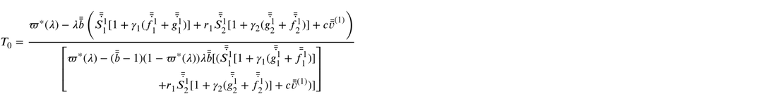
probability of server inactive. Using the normalizing condition, we obtain

T_{0} + T (1) + φ_{1} (1) + φ_{2} (1) + Q_{1} (1) + Q_{2} (1) + D_{1} (1) + D_{2} (1) + S (1) = 1

\bar{\bar{\dot{K_{d}}}} (ħ_{n})

\to

number of customers in the system, where

\bar{\bar{\dot{K_{d}}}} (ħ_{n}) = T_{0} + T_{1} (ħ_{n}) + S (ħ_{n}) + ħ_{n} {φ_{1} (ħ_{n}) + φ_{2} (ħ_{n}) + Q_{1} (ħ_{n}) + Q_{2} (ħ_{n}) + D_{1} (ħ_{n}) + D_{2} (ħ_{n})}

substitute Eq. (51)–(58) we get,

(59)

\bar{\bar{\dot{H_{d}}}} (ħ_{n})

\to

number of customers in the orbit, where

\bar{\bar{\dot{H_{d}}}} (ħ_{n}) = T_{0} + T_{1} (ħ_{n}) + φ_{1} (ħ_{n}) + φ_{2} (ħ_{n}) + Q_{1} (ħ_{n}) + Q_{2} (ħ_{n}) + D_{1} (ħ_{n}) + D_{2} (ħ_{n}) + S (ħ_{n})

substitute Eq. (51)–(58) we get,

(60)

4 Performance measures

Some important measures of effectiveness are derived below.

(i) Let $T (1)$ represents steady-state prob that the server will be inactive during the period.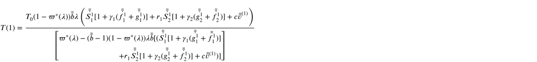

(ii) Let $φ_{1} (1)$ represents the steady-state prob that the server is active.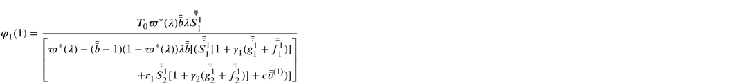

(iii) Let $φ_{2} (1)$ represents the steady-state prob that the server is on NCR.

(iv) Let $Q_{1} (1)$ represents steady-state prob that the server is delaying repair on CR.

(v) Let $Q_{2} (1)$ represents steady-state prob that the server is delaying repair on NCR.

(vi) Let $D_{1} (1)$ represents steady-state prob that the server is repair on CR.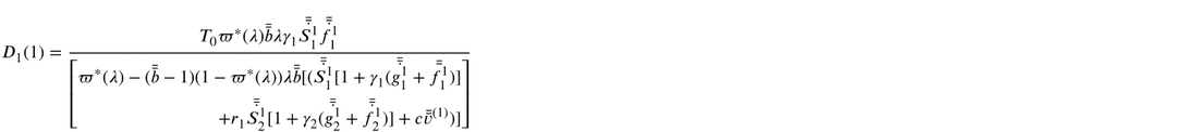

(vii)Let $D_{2} (1)$ represents steady-state prob that the server is delaying repair on NCR.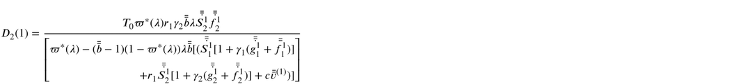

(viii)Let $S (1)$ be the steady-state probability that the server is on MBV.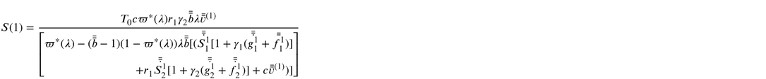

\bar{\bar{L_{s 1}}} \mapsto

average number of customers in the system, is obtained by differentiating Eq. (59) with respect to

ħ_{n}

and evaluating at

ħ_{n} = 1

we get,

\bar{\bar{L_{s 1}}} = \bar{\bar{\dot{K_{d}^{'}}}} (1) and \bar{\bar{L_{q 1}}} = \bar{\bar{\dot{H_{d}^{'}}}} (1)

\bar{\bar{L_{s 1}}} = T_{0} [\frac{D r^{'} N r_{a}^{″} - D r^{″} N r_{a}^{'}}{2 {(D r^{'})}^{2}}]

N r_{a}^{'} = [(1 - \bar{\bar{b}}) + (\bar{\bar{b}} - 1) ϖ^{*} (λ)] + (\bar{\bar{b}} - 1) (1 - ϖ^{*} (λ)) [1 + ϖ^{*} (λ)

+ λ \bar{\bar{b}} (\bar{\bar{\dot{S_{1}^{1}}}} [1 + γ_{1} (\bar{\bar{\dot{g_{1}^{1}}}} + \bar{\bar{\dot{f_{1}^{1}}}})]

+ r_{1} \bar{\bar{\dot{S_{2}^{1}}}} [1 + γ_{2} (\bar{\bar{\dot{g_{2}^{1}}}} + \bar{\bar{\dot{f_{2}^{1}}}})] + c {\bar{\bar{v}}}^{(1)})]

N r_{a}^{″} = (\bar{\bar{b}} - 1) (1 - ϖ^{*} (λ)) \times \{\begin{matrix} {(λ \bar{\bar{b}})}^{2} [(c {\bar{\bar{v}}}^{(2)} + \bar{\bar{\dot{S_{1}^{2}}}} {[1 + γ_{1} (\bar{\bar{\dot{g_{1}^{1}}}} + \bar{\bar{\dot{f_{1}^{1}}}})]}^{2} \\ + γ_{1} ([\bar{\bar{\dot{g_{1}^{2}}}} + \bar{\bar{\dot{f_{1}^{2}}}} + 2 \bar{\bar{\dot{g_{1}^{1}}}} \bar{\bar{\dot{f_{1}^{1}}}}]) \bar{\bar{\dot{S_{1}^{1}}}} + r_{1} ((\bar{\bar{\dot{S_{2}^{2}}}} {[1 + γ_{2} (\bar{\bar{\dot{g_{2}^{1}}}} + \bar{\bar{\dot{f_{2}^{1}}}})]}^{2} \\ + γ_{2} [\bar{\bar{\dot{g_{2}^{2}}}} + \bar{\bar{\dot{f_{2}^{2}}}} + 2 \bar{\bar{\dot{g_{2}^{1}}}} \bar{\bar{\dot{f_{2}^{1}}}}])) \bar{\bar{\dot{S_{2}^{1}}}} + 2 (λ \bar{\bar{b}} (\bar{\bar{\dot{S_{1}^{1}}}} [1 + γ_{1} (\bar{\bar{\dot{g_{1}^{1}}}} + \bar{\bar{\dot{f_{1}^{1}}}})] \\ + r_{1} \bar{\bar{\dot{S_{2}^{1}}}} [1 + γ_{2} (\bar{\bar{\dot{g_{2}^{1}}}} + \bar{\bar{\dot{f_{2}^{1}}}})] + c {\bar{\bar{v}}}^{(1)})) \\ + {(λ \bar{\bar{b}})}^{2} {r_{1} \bar{\bar{\dot{S_{1}^{1}}}} \bar{\bar{\dot{S_{2}^{1}}}} [1 + γ_{1} (\bar{\bar{\dot{g_{1}^{1}}}} + \bar{\bar{\dot{f_{1}^{1}}}})] [1 + γ_{2} (\bar{\bar{\dot{g_{2}^{1}}}} + \bar{\bar{\dot{f_{2}^{1}}}})] \\ + c {\bar{v}}^{(1)} \bar{\bar{\dot{S_{1}^{1}}}} [1 + γ_{1} (\bar{\bar{\dot{f_{1}^{1}}}} + \bar{\bar{\dot{g_{1}^{1}}}})] + c r_{1} {\bar{v}}^{(1)} \bar{\bar{\dot{S_{2}^{1}}}} [1 + γ_{2} (\bar{\bar{\dot{g_{2}^{1}}}} + \bar{\bar{\dot{f_{2}^{1}}}})]} \\ + M^{*} (λ) λ \bar{\bar{b}} (\bar{\bar{\dot{S_{1}^{1}}}} [1 + γ_{1} (\bar{\bar{\dot{g_{1}^{1}}}} + \bar{\bar{\dot{f_{1}^{1}}}})] + r_{1} \bar{\bar{\dot{S_{2}^{1}}}} [1 + γ_{2} (\bar{\bar{\dot{g_{2}^{1}}}} + \bar{\bar{\dot{f_{2}^{1}}}})]))] \end{matrix}\}

\bar{\bar{L_{q 1}}} \mapsto

average number of customers in the orbit, is obtained by differentiating Eq. (60) with respect to

ħ_{n}

and evaluating at

ħ_{n} = 1

we get,

\bar{\bar{L_{q 1}}} = T_{0} [\frac{D r^{'} N r_{b}^{″} - D r^{″} N r_{b}^{'}}{2 {(D r^{'})}^{2}}]

N r_{b}^{'} = (1 - \bar{\bar{b}}) + \bar{\bar{b}} ϖ^{*} (λ) + (\bar{\bar{b}} - 1) (1 - ϖ^{*} (λ) [1 + λ \bar{\bar{b}} (\bar{\bar{\dot{S_{1}^{1}}}}]) [1 + γ_{1} (\bar{\bar{\dot{g_{1}^{1}}}} + \bar{\bar{\dot{f_{1}^{1}}}}) [1 + γ_{2} (\bar{\bar{\dot{g_{2}^{1}}}} + \bar{\bar{\dot{f_{2}^{1}}}})] + c {\bar{\bar{v}}}^{(1)})]

N r_{b}^{″} = (\bar{\bar{b}} - 1) (1 - ϖ^{*} (λ)) \times \{\begin{matrix} {(λ \bar{\bar{b}})}^{2} [(c {\bar{\bar{v}}}^{(2)} + \bar{\bar{\dot{S_{1}^{2}}}} {[1 + γ_{1} (\bar{\bar{\dot{g_{1}^{1}}}} + \bar{\bar{\dot{f_{1}^{1}}}})]}^{2} + γ_{1} ([\bar{\bar{\dot{g_{1}^{2}}}} + \bar{\bar{\dot{f_{1}^{2}}}} + 2 \bar{\bar{\dot{g_{1}^{1}}}} \bar{\bar{\dot{f_{1}^{1}}}}]) \bar{\bar{\dot{S_{1}^{1}}}} \\ + r_{1} (\bar{\bar{\dot{S_{2}^{2}}}} {[1 + γ_{2} (\bar{\bar{\dot{g_{2}^{1}}}} + \bar{\bar{\dot{f_{2}^{1}}}})]}^{2} + γ_{2} [\bar{\bar{\dot{g_{2}^{2}}}} + \bar{\bar{\dot{f_{2}^{2}}}} + 2 \bar{\bar{\dot{g_{2}^{1}}}} \bar{\bar{\dot{f_{2}^{1}}}}]) \bar{\bar{\dot{S_{2}^{1}}}})] \\ + 2 (λ \bar{\bar{b}} (\bar{\bar{\dot{S_{1}^{1}}}} [1 + γ_{1} ({\bar{g_{1}}}^{(1)} + {\bar{f_{1}}}^{(1)})] + r_{1} \bar{\bar{\dot{S_{2}^{1}}}} [1 + γ_{2} ({\bar{g_{2}}}^{(1)} + {\bar{f_{2}}}^{(1)})] \\ + c {\bar{\bar{v}}}^{(1)}) + {(λ \bar{\bar{b}})}^{2} {r_{1} \bar{\bar{\dot{S_{1}^{1}}}} \bar{\bar{\dot{S_{2}^{1}}}} [1 + γ_{1} (\bar{\bar{\dot{g_{1}^{1}}}} + \bar{\bar{\dot{f_{1}^{1}}}})] [1 + γ_{2} (\bar{\bar{\dot{g_{2}^{1}}}} + \bar{\bar{\dot{f_{2}^{1}}}})] \\ + c {\bar{\bar{v}}}^{(1)} \bar{\bar{\dot{S_{1}^{1}}}} [1 + γ_{1} (\bar{\bar{\dot{g_{1}^{1}}}} + \bar{\bar{\dot{f_{1}^{1}}}})] + c r_{1} {\bar{\bar{v}}}^{(1)} \bar{\bar{\dot{S_{2}^{1}}}} [1 + γ_{2} (\bar{\bar{\dot{g_{2}^{1}}}} + \bar{\bar{\dot{f_{2}^{1}}}})]}) \end{matrix}\}

D r^{'} = ϖ^{*} (λ) - λ \bar{\bar{b}} [(\bar{\bar{\dot{S_{1}^{1}}}} [1 + γ_{1} (\bar{\bar{\dot{g_{1}^{1}}}} + \bar{\bar{f_{1}^{1}}})] + r_{1} \bar{\bar{\dot{S_{2}^{1}}}} [1 + γ_{2} (\bar{\bar{\dot{g_{2}^{1}}}} + \bar{\bar{\dot{f_{2}^{1}}}})] + c {\bar{\bar{v}}}^{(1)})]

D r^{''} = - \{\begin{matrix} {(λ \bar{\bar{b}})}^{2} (c {\bar{\bar{v}}}^{(2)} + \bar{\bar{\dot{S_{1}^{2}}}} {[1 + γ_{1} (\bar{\bar{\dot{g_{1}^{1}}}} + \bar{\bar{\dot{f_{1}^{1}}}})]}^{2} + γ_{1} [\bar{\bar{\dot{g_{1}^{2}}}} + \bar{\bar{\dot{f_{1}^{2}}}} + 2 \bar{\bar{\dot{g_{1}^{1}}}} \bar{\bar{\dot{f_{1}^{1}}}}] \bar{\bar{\dot{S_{1}^{1}}}}) \\ + r {\bar{\bar{\dot{S_{2}^{2}}}} {[1 + γ_{2} (\bar{\bar{\dot{g_{2}^{1}}}} + \bar{\bar{\dot{f_{2}^{1}}}})]}^{2} + γ_{2} [\bar{\bar{\dot{g_{2}^{2}}}} + \bar{\bar{\dot{f_{2}^{2}}}} + 2 \bar{\bar{\dot{g_{2}^{1}}}} \bar{\bar{\dot{f_{2}^{1}}}}] \bar{\bar{\dot{S_{2}^{1}}}}} \\ + 2 {(1 - M^{*} (λ)) [(λ \bar{\bar{b}}) \bar{\bar{\dot{S_{1}^{1}}}} [1 + γ_{1} (\bar{\bar{\dot{g_{1}^{1}}}} + \bar{\bar{\dot{f_{1}^{1}}}})] + r_{1} λ \bar{\bar{b}} \bar{\bar{\dot{S_{2}^{1}}}} [1 + γ_{2} (\bar{\bar{\dot{g_{2}^{1}}}} \\ + \bar{\bar{\dot{f_{2}^{1}}}})] + c {\bar{\bar{v}}}^{(1)}] + r_{1} λ {\bar{\bar{b}}}^{2} \bar{\bar{\dot{S_{1}^{1}}}} \bar{\bar{\dot{S_{2}^{1}}}} [1 + γ_{1} (\bar{\bar{\dot{g_{1}^{1}}}} + \bar{\bar{\dot{f_{1}^{1}}}})] [1 + γ_{2} (\bar{\bar{\dot{g_{2}^{1}}}} + \bar{\bar{\dot{f_{2}^{1}}}})] \\ + c {\bar{\bar{v}}}^{(1)} {(λ \bar{\bar{b}})}^{2} ([1 + γ_{1} (\bar{\bar{\dot{g_{1}^{1}}}} + \bar{\bar{\dot{f_{1}^{1}}}})] + r_{1} [1 + γ_{2} (\bar{\bar{\dot{g_{2}^{1}}}} + \bar{\bar{\dot{f_{2}^{1}}}})])} \end{matrix}\}

Applying Little’s formula we get

\bar{\bar{W_{s 1}}} = \frac{\bar{\bar{L_{s 1}}}}{λ}, \bar{\bar{W_{q 1}}} = \frac{\bar{\bar{L_{q 1}}}}{λ}

5 Special cases

Here we consider all the three special cases without balking.

Case(i): No NCR, and $r_{1} = 0$ $\begin{matrix} \bar{\bar{\dot{K_{d}}}} (ħ_{n}) = T_{0} \{\begin{matrix} \frac{U_{1}^{*} ({\bar{\bar{Λ}}}_{a} (ħ_{n})) (ħ_{n} - 1)}{ħ_{n} - [ϖ^{*} (λ) + ħ_{n} (1 - ϖ^{*} (λ))] U_{1}^{*} ({\bar{\bar{Λ}}}_{a} (ħ_{n})) [(1 - c) + c B^{*} h_{11} (ħ_{n})]} \end{matrix}\} \end{matrix}$ Where $T_{0} = \frac{ϖ^{*} (λ) - λ (\bar{\bar{\dot{S_{1}^{1}}}} (1 + γ_{1} (\bar{\bar{\dot{g_{1}^{1}}}} + \bar{\bar{\dot{f_{1}^{1}}}})) + c {\bar{\bar{v}}}^{(1)})}{ϖ^{*} (λ)}$

Case(ii): Let c = 1, $γ_{1} = γ_{2} = 0$ and $ϖ^{*} (λ) \to 1$ $\begin{matrix} \bar{\bar{\dot{K_{d}}}} (ħ_{n}) = T_{0} \{\begin{matrix} \frac{U_{1}^{*} (h_{11} (ħ_{n})) (ħ_{n} - 1) [(\bar{r_{1}} + r_{1} U_{2}^{*} (h_{11} (ħ_{n})))]}{ħ_{n} - U_{1}^{*} (h_{11} (ħ_{n})) [(\bar{r_{1}} + r_{1} U_{2}^{*} (h_{11} (ħ_{n})) B^{*} (h_{11} (ħ_{n})))]} \end{matrix}\} \end{matrix}$

Where $T_{0} = 1 - λ (\bar{\bar{\dot{S_{1}^{1}}}} + \bar{\bar{\dot{S_{2}^{1}}}} + {\bar{\bar{v}}}^{(1)})$

Case(iii): No vacation, no NCR, and $γ_{1} = γ_{2} = 0$

The below obtained expression concedes with Gomez-Corral (1999) $\begin{matrix} \bar{\bar{\dot{K_{d}}}} (ħ_{n}) = T_{0} \{\begin{matrix} \frac{U_{1}^{*} (h_{11} (ħ_{n})) (ħ_{n} - 1)}{ħ_{n} - U_{1}^{*} (h_{11} (ħ_{n})) [ϖ^{*} (λ) + ħ_{n} (1 - ϖ^{*} (λ))]} \end{matrix}\} \end{matrix}$

Where $T_{0} = \frac{ϖ^{*} (λ) - λ \bar{\bar{\dot{S_{1}^{1}}}}}{ϖ^{*} (λ)}$

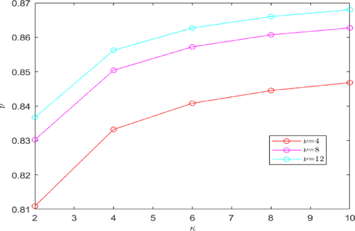
6 Numerical interpretations

The goal of this section is to analyze the influence of several variables on various system performance measures. The arbitrary values that are considered for the parameters are selected in such a way that they may meet the criterion that the system is stable. This condition is fulfilled when the parameters have consistent values. The retrial, service, MBV, and repair time are all considered as exponential distribution, $f (ħ_{l}) = Θ e^{- Θ ħ_{l}}, ħ_{l} > 0$ . This confirms that these times are realistic and consistent.

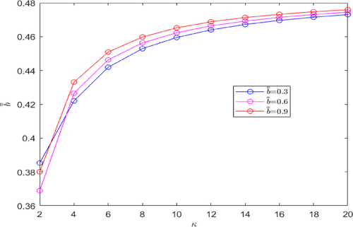
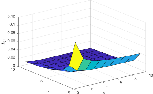
Fig. 1 and Fig. 2 shows that as retry rate ( $κ$ ) escalates, the $T_{0}$ also escalate. In Fig. 3 if retry and vacation escalates, $\bar{\bar{L_{q 1}}}$ decreases. In Fig. 4 also if retry and service (compulsory) escalates, $\bar{\bar{L_{q 1}}}$ decreases.

7 Conclusion

In this work, we have presented a single server retrial queueing system with balking under MBV (Modified Bernoulli vacation policy), where the busy server is prone to both failure and repair. Using the supplementary variable method (SVM), the probability generating functions for the number of users in the system when it is idle, occupied, MBV, and repair are presented. Various significant system performance metrics such as expected number of customers in an orbit and the system and server utilization have also been analyzed. Numerical illustrations are presented to demonstrate the analytical findings of the model. Future research of this paper could focus on expanding this queueing model to include modified working vacation policies, randomized policies, setup time and cost estimation. CCM (Cloud Computing Model), PSN (Packet Switched Network) for the transfer of packets in a network, and WSN (Wireless Sensor Network) for choosing and maintaining routes are some of the practical and real-world applications of this model.

Declaration of competing interest

The authors declare that there is no conflict of interest.

References

Arivudainambi D., Godhandaraman P., . A batch arrival retrial queue with two phases of service, feedback and K optional vacations. Appl. Math Sci.. 2012;6(22):1071-1087.
[Google Scholar]
Artalejo J.R., Choudhury G., . Steady state analysis of an $M / G / 1$ queue with repeated attempts and two-phase service. Qual. Technol. Quant. Manag.. 2004;1(2):189-199.
[Google Scholar]
Bouchentouf A.A., Boualem M., Cherfaoui M., Medjahri L., . Variant vacation queueing system with bernoulli feedback, balking and server’s states-dependent reneging. Yugoslav J. Oper. Res.. 2021;31(4):557-575.
[Google Scholar]
Boussaha, Z., Oukid, N., Zeghdoudi, H., Soualhi, S., Djellab, N., 2022. On the $m / g / 1$ feedback retrial queueing with orbital search of customers.
Boxma O.J., Vlasiou Maria, . On queues with service and interarrival times depending on waiting times. Queueing Syst.. 2007;56(3):121-132.
[Google Scholar]
Choudhury G., Deka K., . An $M / G / 1$ retrial queueing system with two phases of service subject to the server breakdown and repair. Perform. Eval.. 2008;65(10):714-724.
[Google Scholar]
Choudhury G., Madan K.C., . A two-stage batch arrival queueing system with a modified Bernoulli schedule vacation under N-policy. Math. Comput. Model.. 2005;42(1):71-85.
[Google Scholar]
Dimitriou I., . A two-class queueing system with constant retrial policy and general class dependent service times. Eur. J. Oper. Res.. 2018;270(3):1063-1073.
[Google Scholar]
Doshi B., . Queueing systems with vacations-a survey. Queueing Syst.. 1986;1(1):29-66.
[Google Scholar]
Falin G.I., Templeton T.G.C., . Retrial Queues. London: Chapman and Hall; 1997.
Gomez-Corral A., . Stochastic analysis of single server retrial queue with the general retrial times. Nav. Res. Logist.. 1999;46(5):561-581.
[Google Scholar]
Jain M., Agarwal Praveen.kumar., . N-policy for state-dependent batch arrival queueing system with l-stage service and modified Bernoulli vacation. Qual. Technol. Qual. Manag.. 2010;7(3):215-230.
[Google Scholar]
Ke J.C., Wu C.U., Zhang Z.G., . Recent developments in vacation models: a short survey. Int. J. Oper. Res.. 2010;7(4):3-8.
[Google Scholar]
Kerner Y., . The conditional distribution of the residual service time in the $M / G / 1$ queue. Stoch. Models. 2008;24(3):364-375.
[Google Scholar]
Lan S., Tang Y., . An unreliable discrete-time retrial queue with probabilistic preemptive priority, balking customers and replacements of repair times. AIMS Math.. 2020;5(5):4322-4344.
[Google Scholar]
Legros B., . Dimensioning a queue with state-dependent arrival rates. Comput. Oper. Res.. 2021;128(10):51-79.
[Google Scholar]
Legros B., . The principal–agent problem for service rate event-dependency. European J. Oper. Res.. 2022;297(3):949-963.
[Google Scholar]
Madheswari S.P., Krishnakumar B., Suganthi P., . Analysis of $M / G / 1$ retrial queues with second optional service and customer balking under two types of Bernoulli vacation schedules. Operations research. 2019;53(2):415-443.
[Google Scholar]
Nandhini S., . Low Latency Weighted Fair Queuing for Real time flows with Differential Packet Dropping. Vol. 8. No. 22. 2013. p. :1-5.
Wang J., Li J., . A single server retrial queue with general retrial times and two phase service. Jrl. Syst. Sci. Complex.. 2009;22(2):291-302.
[Google Scholar]