A semi-parametric estimator of the quantile residual life for heavily censored data

1 Introduction

In many fields such as epidemiology, biology, medicine, and survival analysis, the researcher's interest is on time to event data, e.g., the survival time of a creature or time of tumor recurrence. The most familiar measure for induction and analyzing such data is the survival function, which for every time t ≥ 0 computes the probability of the event to occur beyond time t. The p-quantile residual life (p-QRL) function, 0 < p < 1, is another relevant measure in this context providing an intuitive meaning. For example, in the case p = 0.5, we have a median residual life which at time t captures the remaining time that half of the survived population at t will experience the event. This fact that unlike the survival function, the p-QRL is expressed in the time units by which the observations are measured makes its interpretation easier.

Besides, in reliability analysis, the p-QRL measure is quite useful for describing the lifetime of manufactured devices. For instance, it is very likely for some devices to fail in the early stages of their work. It is the case especially when the failure rate has a bathtub shape. Then we can consider a burn-in time t₀ that every produced device should pass before releasing to field operation. We can find such t₀ that maximizes the p-QRL function. For more details, we refer to Conboy et al. (2020).

Sometimes, time events may be invisible due to some censoring mechanism which cannot be naturally avoided. During the study, some items may be lost to follow-up before experiencing the event or reaching the end-time of the study. They are said to be right-censored. However, items passing the end-time of the study are referred to be Type I censored.

Given a right-censored data set, the survival function can be estimated using Kaplan-Meier (KM) estimator proposed by Kaplan and Meier (1958). The KM survival plot, which summarizes the possibly censored data graphically, has been vastly used in the aforementioned areas. On the other hand, taking account of right censoring, many authors focused on the problem of estimating the p-QRL function. Among them, we refer to Jeong et al. (2008), Franco-Pereira and de Uña-Álvarez (2013), Jeong and Fine (2013), Lin et al. (2015), Zhang et al. (2015), and Lin et al. (2016).

One drawback in right-censored data corresponds to the case that the upper tail and especially last observations are censored. In this case, the KM survival estimator does not vanish to zero in the support tail. Thus, the inverse of the survival function at small values will not be estimable by the KM estimator. Therefore, we cannot estimate the p-QRL function especially at large values (cf. Franco-Pereira and de Uña-Álvarez (2013)). The results of many types of research consist of highly censored data sets in which major of their large observations are censored. For such data sets, we may not estimate the p-QRL function, namely, qp(t), (for example, the median residual life) even at rather small ts. Therefore, our idea is to provide an approach to estimate the p-QRL function for all t values.

In this paper, we propose a new semi-parametric method for estimating the p-QRL function that overcomes the problem of dealing with high censored lifetimes. It applies the KM estimator of the survival function in a proper threshold time u, and the generalized Pareto distribution (GPD) as an approximated tail model (Coles (2001)). The approximation of the tail model is motivated by the results of the extreme value theory, refer to Castillo et al. (2005) and Coles (2001). Then, the uncensored observations in the tail (which we suppose to be greater than the threshold u) are used to provide the maximum likelihood estimation of the model parameters.

The paper has been organized as follows. Section 2 provides preliminaries and states the problem. In Section 3, the new estimator of the p-QRL function has been proposed. The attributes of this estimator are investigated through a simulation study in Section 4. In Section 5, the results of a research investigation of the effect of some treatments on the colon recurrence time are considered. Then the first quartile residual life (0.25-QRL) and the median residual life functions are estimated. Finally, a conclusion is drawn in Section 6.

2 Preliminaries: Non-parametric estimation of $\mathit{p}$-QRL

Let the random variable $T$ which represents the lifetime of an object follows the survival function $S\left(t\right)=P(T>t)$. The $p$-QRL function is defined as

When the last observation has not been censored, the estimator $\left(2\right)$ is well-defined for all $t\le X^{\ast }$. Otherwise, it is not defined for all values $t>t^{\ast }$ where $t^{\ast }$ stands for ${\widehat{S}}^{-1}\left(\frac{1}{\stackrel{-}{p}}\widehat{S}\left(X^{\ast }\right)\right)$. When $t>t^{\ast }$, $\stackrel{-}{p}\widehat{S}\left(t\right)<\widehat{S}\left(X^{\ast }\right)$ that is $\stackrel{-}{p}\widehat{S}\left(t\right)$ falls below the computable range of the inverse of KM survival function. Fig. 1 explains the issue graphically.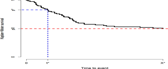

Close

Fig. 1

This illustrative plot shows that when large observations have been censored the QRL function $q_p$ ($t$) is not estimable for $t>t^{\ast }$ by the inverse of the KM survival function. Here, $p^{\ast }$ and $p_0$ equal to $\frac{1}{p}$ $\widehat{\mathrm{S}}$($X^{\ast }$) and $\widehat{\mathrm{S}}$($X^{\ast }$) respectively.

Export to PPT

3 Semi-parametric estimation of $\mathit{p}$-QRL

This section aims to propose a semi-parametric estimator of $q_p\left(t\right)$ for $t>t^{\ast }$. Note that if $0<p_2<p_0<p_1<1$, then

Consider an arbitrary sequence of i.i.d. random variables T₁,T₂,… following the same distribution of T and let $M_n$ be maximum of the first $n$ elements of this sequence. Let there exist sequences $a_n>0$ and $b_n$ of constants such that the normalized random sequence $a_n(M_n-b_n)$ converges weakly to non-degenerate distribution $G$. Then, $G$ accommodates GEV

On the other hand, the max-stability property of the GEV model states that $G^{\frac{1}{n}}\left(a_n(t-b_n)\right)$ equals with $G\left(a_n^{\text{'}}(t-b_n^{\text{'}})\right)$. Thus, for $t\ge u$, $F_T\left(t\right)$ belongs to this family too, notationally, $F_T\left(t\right)=G\left(t\right)$, $t\ge u$. In the light of the preceding discussion, we can approximate $S_u\left(t\right)$ for some threshold $u$ by:$$S_u\left(t\right)=\frac{S(t+u)}{S\left(u\right)}\approx \frac{\stackrel{-}{G}(t+u)}{\stackrel{-}{G}\left(u\right)}=\frac{1-\mathrm{e}\mathrm{x}\mathrm{p}\left\{-{\left[1+\xi \left(\frac{u+t-\mu }{\sigma }\right)\right]}^{-\frac{1}{\xi }}\right\}}{1-\mathrm{e}\mathrm{x}\mathrm{p}\left\{-{\left[1+\xi \left(\frac{x-\mu }{\sigma }\right)\right]}^{-\frac{1}{\xi }}\right\}}.$$

Since $u$ is sufficiently large, we have$$\frac{1-\mathrm{e}\mathrm{x}\mathrm{p}\left\{-{\left[1+\xi \left(\frac{u+t-\mu }{\sigma }\right)\right]}^{-\frac{1}{\xi }}\right\}}{1-\mathrm{e}\mathrm{x}\mathrm{p}\left\{-{\left[1+\xi \left(\frac{x-\mu }{\sigma }\right)\right]}^{-\frac{1}{\xi }}\right\}}\approx \frac{{\left[1+\xi \left(\frac{u+t-\mu }{\sigma }\right)\right]}^{-\frac{1}{\xi }}}{{\left[1+\xi \left(\frac{x-\mu }{\sigma }\right)\right]}^{-\frac{1}{\xi }}}.$$

Then, by simplifying the right side of this approximation, it follows that

• $\xi <0$: light tail with finite upper bound $-\frac{{\sigma }_u}{\xi }$.

• $\xi =0$: exponential tail.

• $\xi >0$: heavy tail.

When $\xi >\frac{1}{s}$, the $s$th moment of GPD is infinite. So, when we are confident of finite mean and/or variance it may be useful to restrict the parameter space by $0<\xi \le 1\mathrm{a}\mathrm{n}\mathrm{d}/\mathrm{o}\mathrm{r}0.5$. However, such restriction is not recommended in a neat semi-parametric framework. For GDP$\left(5\right)$, the inverse of the survival function equals with

To implement the method for censored data, let $T_i$, $C_i^{\text{'}}$ and $T^{\ast }$ be true survival time, random right censoring time, and a constant time presenting end of the study, respectively. Taking $C_i=\mathrm{m}\mathrm{i}\mathrm{n}(C_i^{\text{'}},T^{\ast })$, we observe $X_i=\mathrm{m}\mathrm{i}\mathrm{n}(T_i,C_i)$ and ${\delta }_i=I(T_i\le C_i)$. To estimate $q_p\left(t\right)$ for $t>t^{\ast }$, we suggest the following steps.

• At first we should select a proper value for $u$ which is a trade-off between the accuracy of the tail model approximation and the share of the observations available for estimating the model parameters. Large values of $u$ improve the approximation of the model but limit the volume of the observations for estimation of the parameters. Yet, there is not any standard approach for finding an optimum value for $u$. Nevertheless, it seems that the $80$ percent quantile of the observed (uncensored) times be a proper value for threshold $u$. That is $20$ percent of observed and uncensored events lie between $u$ and $T^{\ast }$ (see Alvarez-Iglesias et al. (2015) for a similar discussion).

• Construct new sample $x_i=t_i-u$ for all censored or uncensored observations $t_i$ grater than $u$ and let $k$ denote the count of them. Applying this data set, we obtain the maximum likelihood estimation of the parameters of GPD model $\left(5\right)$. The likelihood function is

• Now, in the light of Relations $\left(3\right)$ and $\left(6\right)$, we propose the estimator

Variance (bias) of this estimator is comprised of variation (bias) due $u$, and ${\widehat{S}}_u^{-1}(\stackrel{-}{p}\widehat{S}\left(t\right)/\widehat{S}\left(u\right))$ along with their covariance and seems to be more complicated than to be expressed by a closed expression. In the case of the heavy tail of the true lifetime model which causes that $\widehat{\xi }>0$, it’s variance increases with $t$. Fortunately, we can use the bootstrap method to estimate its bias and variance and in turn approximate confidence intervals. However, simulation studies heuristically imply that bias and variance reduce strongly by sample size.

4 Simulation study

To design a simulation framework, we consider gamma, log-normal, and Weibull models along with four censoring schemas. Both right censoring and Type I censoring have been taken in account. Once the model and the censoring scheme determined, $r=100$ replicates of samples of sizes $n=500$ and $1000$ have been drawn and censored. Then for two values $p=0.5$ (corresponding to the median residual life function) and $p=0.75$ the proposed estimator ${\widehat{q}}_p\left(t\right)$ has been computed by each of $r$ replicates. For each replicates the bias is computed by the difference ${\widehat{q}}_p\left(t\right)-q_p\left(t\right)$. We report their mean and standard deviation as bias and sd in Tables 1–3. In addition, $M{\widehat{q}}_p$ that shows the mean of the estimation values ${\widehat{q}}_p\left(t\right)$ has been entered in the tables.

To provide censored random samples, some proper combinations of right censoring and Type I censoring have been selected. Let ${\alpha }_1$ and ${\alpha }_2$ represent the proportions of Type I censoring and random right censoring respectively. The simulation process starts withdrawing a sample of size $n$ from the true model that is the distribution of $T$ following survival function $S$. We take the distribution of the right censoring random variable $C$ to be uniform on the interval $(0,M)$. Moreover, according to type I censoring, the observations will be censored if they are greater than $T^{\ast }$. For fixed values ${\alpha }_1$ and ${\alpha }_2$, we should compute $M$ and $T^{\ast }$ through the equations $P(C<\mathrm{m}\mathrm{i}\mathrm{n}\{T,T^{\ast }\})={\alpha }_2$ and $P(\{T^{\ast }<T<C\}\cup \{T^{\ast }<C<T\})={\alpha }_1$. It is straightforward to show that these equations can be simplified to the system equations$$\left\{\begin{array}{c}S\left(T^{\ast }\right)(M-T^{\ast })=M{\alpha }_1,\hfill \\ \underset{0}{\stackrel{T^{\ast }}{\int }}S\left(x\right)dx=M{\alpha }_2,\hfill \end{array}\right.$$which can be solved in terms of $M$ and $T^{\ast }$ by standard numerical methods. Then, we can pursue the procedure according to the bellow steps.

• Generate a random sample $t_1,t_2,\cdots ,t_n$ from the true model with the survival function $S$.

• Generate a random sample $c_1,c_2,\cdots ,c_n$ of uniform $(0,M)$ as random censoring times.

• Compute the observable data $x_i=\mathrm{m}\mathrm{i}\mathrm{n}\{t_i,c_i,T^{\ast }\}$ and ${\delta }_i=I(t_i\le c_i,t_i\le T^{\ast })$ for $i=1,2,\cdots ,n$.

• Repeat steps 1 to 3 $r$ times.

• Let $t_{0j}$ be the maximum observed (uncensored) lifetime of the sample in the $j$th replication, $j=1,2,\cdots ,r$. Then, take $t_0$ to be the mean of $t_{0j}$. Of course, $t_0$ is suitable for applying in the simulation, since it is expected that ${\widehat{S}}^{-1}\left(\stackrel{-}{p}\widehat{S}\left(t_0\right)\right)$ will not be computed by the KM estimator $\widehat{S}$.

• For each replication, compute ${\widehat{q}}_p\left(t_0\right)$ introduced by $\left(7\right)$.

Results of simulations have been gathered in Tables 1–3. All tables agree on the fact that the bias and sd values show a strong reduction from $p=0.75$ to $0.5$.

5 Applications

Moertel et al (1995) reported a data set related to one trial for investigation of the effectiveness of Fluorouracil (5-FU) and Levamisole (Lev) in reducing the recurrence rate of stage B/C colon cancer. The trial involves three treatments for Observation (Obs), Levamisole (Lev), and Levamisole plus 5-FU (Lev + 5-FU). Under right censoring, for every person, both events of recurrence of cancer and death have been recorded. We focus on the recurrence times which near $50$ percent of them have been censored. For each of the three treatments and the overall data, the KM survival function has been drawn in Fig. 2, which reveals high censoring rates.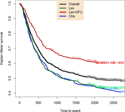

Close

Fig. 2

The KM survival plot for three treatments and the overall data. Every censored item is included by a+.

Export to PPT

We are interested in the estimation of the first QRL function and the median residual life function respectively corresponding to $p=0.25$ and $0.5$. As before, let $t^{\ast }$ stand for the minimum of $t$ values where the QRL can not be computed directly by inverting the KM survival function. Values of $t^{\ast }$ computed for these data sets have been gathered in Table 4.

The first quartile residual life function and the median residual life function have been plotted in Figs. 3 and 4$,$ respectively. For $t<t^{\ast }$ these functions have been estimated by $\left(2\right)$ and have been plotted by a thinner line.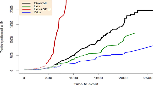

Close

Fig. 3

The first quartile residual life function for three treatments and the overall data.

Export to PPT

Close

Fig. 4

The median residual life function for three treatments and the overall data.

Export to PPT

These figures distinguish larger median residual life and first quartile residual life functions for Lev + 5-FU treatment, which are even noticeably above the QRL functions related to overall data. However, for two treatments Obs and Lev, both of these QRL functions are comparable and lie below the QRL functions of the overall group.

6 Conclusion

The p-quantile residual life function summarizes the lifetime data in a useful and simple concept and in units of time. For uncensored data or when the upper tails of the observations are not censored, this function can be estimated by applying the well-known Kaplan-Meier survival estimator. However, when research terminates in heavy right-censored lifetime data, which is the case of many biomedical and survival studies, the p-quantile residual life function is not estimable in this way. In the current investigation, we proposed a novel semi-parametric estimator of the p-quantile residual life function in such cases. The proposed estimator has been examined by a simulation study and applied to a real lifetime data set in the sequel.

Funding

This Project was funded by the National Plan for Science, Technology, and Innovation (MAARIFAH), King Abdulaziz City for Science and Technology, Kingdom of Saudi Arabia, Award Number (14-MAT2052-02).

References

- Summarising censored survival data using the mean residual life function. Stat. Med.. 2015;34:1965-1976.
- [Google Scholar]
- Extreme Value and Related Models with Applications in Engineering and Science. Hoboken, New Jersey: Wiley Series in Probability and Statistics Wiley; 2005.
- An Introduction to Statistical Modeling of Extreme Values. London: Springer; 2001.
- Using business analytics to enhance dynamic capabilities in operations research: a case analysis and research agenda. Eur. J. Operation. Res. Elsevier. 2020;281(3):656-672.
- Counting Processes and Survival Analysis. New York: Wiley; 1991.
- Estimation of a monotone percentile residual life function under random censorship. Biom. J.. 2013;55:52-67.
- Nonparametric inference on cause-specific quantile residual life. Biom. J.. 2013;55:68-81.
- Nonparametric inference on median residual life function. Biometrics. 2008;64:157-163.
- Nonparametric estimation from incomplete observations. J. Am. Stat. Assoc.. 1958;53:457-481.
- Inference on quantile residual life function under right-censored data. J. Nonparametr. Stat.. 2016;28:617-643.
- Conditional quantile residual lifetime models for right-censored data. Lifetime Data Anal.. 2015;21:75-96.
- Fluorouracil plus Levamisole as an effective adjuvant therapy after resection of stage II colon carcinoma: a final report. Ann. Intern. Med.. 1995;122:321-326.
- Smoothed estimator of quantile residual lifetime for right-censored data. J. Syst. Sci. Complex. 2015;28:1374-1388.