A semi-analytical iterative technique for solving chemistry problems

Majeed Ahmed AL-Jawary; Russell Khalil Raham

doi:10.1016/j.jksus.2016.08.002

View/Download PDF

Buy Reprints

PDF

Translate this page into:

29 (

); 320-332

doi:

10.1016/j.jksus.2016.08.002

A semi-analytical iterative technique for solving chemistry problems

Majeed Ahmed AL-Jawary^{^a,⁎}, Russell Khalil Raham^{^b}

a Head of Department of Mathematics, College of Education for Pure Science (Ibn AL-Haytham)/Baghdad University, Baghdad, Iraq

b Department of Mathematics, College of Education for Pure Science (Ibn AL-Haytham)/Baghdad University, Baghdad, Iraq

⁎Corresponding author.

Received: 2016-7-18, Accepted: 2016-8-15, Published: 2016-07-01

Disclaimer:
This article was originally published by Elsevier and was migrated to Scientific Scholar after the change of Publisher.

Peer review under responsibility of King Saud University.

Abstract

The main aim and contribution of the current paper is to implement a semi-analytical iterative method suggested by Temimi and Ansari in 2011 namely (TAM) to solve two chemical problems. An approximate solution obtained by the TAM provides fast convergence. The current chemical problems are the absorption of carbon dioxide into phenyl glycidyl ether and the other system is a chemical kinetics problem. These problems are represented by systems of nonlinear ordinary differential equations that contain boundary conditions and initial conditions. Error analysis of the approximate solutions is studied using the error remainder and the maximal error remainder. Exponential rate for the convergence is observed. For both problems the results of the TAM are compared with other results obtained by previous methods available in the literature. The results demonstrate that the method has many merits such as being derivative-free, and overcoming the difficulty arising in calculating Adomian polynomials to handle the non-linear terms in Adomian Decomposition Method (ADM). It does not require to calculate Lagrange multiplier in Variational Iteration Method (VIM) in which the terms of the sequence become complex after several iterations, thus, analytical evaluation of terms becomes very difficult or impossible in VIM. No need to construct a homotopy in Homotopy Perturbation Method (HPM) and solve the corresponding algebraic equations. The MATHEMATICA® 9 software was used to evaluate terms in the iterative process.

Keywords

Chemical problems

Systems of ordinary differential equations

Approximate solutions

The maximal error remainders

Show Related Articles from PubMed

1 Introduction

In practical life, there are many phenomena in Chemistry, Mechanics, Biology, Physics and Fluid Dynamics can be represented by either linear or nonlinear differential equations. In Chemistry for example, the condensations of carbon dioxide and phenyl glycidyl ether and chemical kinetics problem are represented by systems of nonlinear ordinary differential equations (ODEs).

Carbon dioxide (CO₂) is used in many fields such as plant photosynthesis, fire extinguishers, and removing caffeine from coffee. Carbon dioxide is generally a beneficial gas which consists of one carbon atom and two oxygen atoms (Duan et al., 2015; AL-Jawary and Radhi, 2015; Muthukaruppan et al., 2012 ). On the other hand the chemical kinetics system introduced by Robertson in 1966 is a nonlinear model (Aminikhah, 2011; Ganji et al., 2007).

Many types of ODEs are solved either analytically or numerically for examples: the Variational Iteration Method (VIM) is used to solve the nonlinear settling particle equation of Motion (Ganji, 2012). The He’s Homotopy Perturbation Method (HPM), which does not need small parameter in the equation is implemented for solving the nonlinear Hirota–Satsuma coupled KdV partial differential equation (Ganji and Rafei, 2006). Deniz and Bildik (2014) have implemented the comparison of Adomian Decomposition Method (ADM) and Taylor matrix method for solving different kinds of partial differential equations. Also, Bildik and Deniz (2015a) have used both Taylor collocation and ADM for solving systems of ordinary differential equations. Moreover, Bildik and Deniz (2015b) have successfully implemented taylor collocation method, lambert w function and VIM for solving systems of delay differential equations. Wazwaz (2005) has used the ADM for solving the Bratu-type equations.

Several methods have been used to solve the system of condensations of carbon dioxide and phenyl glycidyl ether and obtained analytical approximate solutions such as, Adomian Decomposition Method (ADM) was applied to simple steady-state condensations of CO₂ and PGE (Duan et al., 2015; Muthukaruppan et al., 2012), the VIM (AL-Jawary and Radhi, 2015) and the iterative method (DJM) (AL-Jawary et al., 2016).

On the other hand, the chemical kinetics problem is solved by many methods and the solution is obtained as approximate solutions. Ganji et al. (2007) have successfully implemented both the VIM and HPM for the system. Khader (2013) has used the so-called Picard–Pade technique to solve the system. Also, Aminikhah (2011) has used (HPM) to solve the system. Moreover, Matinfar et al. (2014) have applied the homotopy analysis method (HAM) and the solutions obtained by HAM have high accuracy in comparison with HPM and VIM introduced in Ganji et al. (2007).

Furthermore, some analytic and approximate methods have recently been used and implemented to solve different chemical and physics problems and other sciences for examples: Differential Transform Method (DTM) has been used to solve fourth order singularly perturbed two-point boundary value problems which occur in chemical reactor theory (El-Zahar, 2013). Matinfar et al. (2015) have found that the interaction of electromagnetic wave with electron is solved by VIM. In Vazquez-Leal et al. (2015) the authors present a comparison of Homotopy Perturbation Method (HPM), Nonlinearities Distribution Homotopy Perturbation Method (NDHPM), Picard, and Picard–Padé methods to solve Michaelis–Menten equation. Also, Cá zares-Ramı́rez and Espinosa-Paredes (2016) the authors studied the behavior of heat and mass transfer during hydrogen generation in the core of the boiling water reactor (BWR). Makinde (2007a,b) has implemented the ADM to compute an approximation to the solution of the non-linear system of differential equations governing the SIR epidemic model and the ratio-dependent predator–prey system with constant effort harvesting. In addition, Makinde (2009) has successfully applied the ADM coupled with Padé approximation technique and VIM to approximate the solution of the governing non-linear systems of a mathematical model that describes the dynamics of re-infection under the assumption that the vaccine induced immune protection may wane over time.

Recently, Temimi and Ansari (2011a) have introduced the semi-analytical iterative technique in 2011 for solving nonlinear problems. The TAM is used for solving many differential equations, such as nonlinear second order multi-point boundary value problems (Temimi and Ansari, 2011b), nonlinear ordinary differential equations (Temimi and Ansari, 2015), korteweg–de vries equations (Ehsani et al., 2013) and the results obtained from the method indicate that the TAM is accurate, fast, appropriate, time saver and has a higher convergence.

In this paper, the TAM will be applied to solve two chemical problems. The first problem is a nonlinear system of the concentrations of carbon dioxide and phenyl glycidyl ether. The other is a chemical kinetics problem which is also represented by a nonlinear system of ODEs. Special discussion is given for the study of the convergence based on Temimi and Ansari (2015), the error analysis of the method (TAM), the error remainders and the convergence of the TAM will be discussed.

This paper has been organized as follows: In Section 2, the steady-state of the chemical problems will be introduced. In Section 3, the basic idea of TAM is presented and discussed. In Section 4, solving the chemical problems by the TAM will be given. In Section 5, the convergence and error analysis are introduced and discussed. In Section 7, the numerical simulation will be illustrated and discussed. Finally, the conclusion in Section 8 will be given.

2 Steady-state of the chemical problems

2.1

2.1 Condensations of carbon dioxide and phenyl glycidyl ether

The mathematical formulation of the concentrations of Carbon dioxide and phenyl glycidyl ether can be shown as follows (Muthukaruppan et al., 2012):

The comprehensive reaction between CO₂ and PGE for forming (5-membered cyclic carbonate) can be presented as

(1)

where R is a functional group of –CH₂–O–C₆H₅. The comprehensive reaction of Eq. (1) consists the two following successive steps: (1) the reaction between PGE (A₂) and THA-CP-MS41(QX) for forming (E₁); (2) the reaction between (E₁) and CO₂ (A₁) for forming (QX) and 5-membered cyclic carbonate (C):

(2)

A_{2} + QX ⇌_{b_{2}}^{b_{1}} E_{1}

(3)

A_{1} + E_{1} \overset{b_{3}}{\to} C + QX

At steady state condition, the successively chemical reaction rate of CO₂ for forming $E_{1}$ is given as follows:

(4)

r_{A_{1}, cond} = \frac{C_{A_{2}} S_{t}}{\frac{1}{b_{1}} + \frac{1}{B b_{3} C_{A_{1}}} + \frac{C_{A_{2}}}{b_{3} C_{A_{1}}}}

where,

C_{A_{1}}

and

C_{A_{2}}

are the concentrations CO₂ and PGE respectively,

S_{t}

is the surface area of catalyzer.

B

is the reaction balance constant, the constant

b_{1}

in Eq. (2), is the forward reaction rate constant and in Eq. (3)

b_{3}

is the forward reaction rate constant. The mass equilibrium of CO₂ and PGE using the film theory escorted by the successively chemical reactions are presented as follows (Choe et al., 2010):

(5)

D_{A_{1}} \frac{d^{2} C_{A_{1}}}{{dz}^{2}} = \frac{C_{A_{2}} S_{t}}{\frac{1}{b_{1}} + \frac{1}{B b_{3} C_{A_{1}}} + \frac{C_{A_{2}}}{b_{3} C_{A_{1}}}}

(6)

D_{A_{2}} \frac{d^{2} C_{A_{2}}}{{dz}^{2}} = \frac{C_{A_{2}} S_{t}}{\frac{1}{b_{1}} + \frac{1}{B b_{3} C_{A_{1}}} + \frac{C_{A_{2}}}{b_{3} C_{A_{1}}}}

where

z

is the distance and

D_{A_{1}}

and

D_{A_{2}}

are the diffusivity of CO₂ and PGE successively. The boundary conditions are:

(7)

C_{A_{1}} = C_{A_{1 i}}, \frac{{dC}_{A_{2}}}{dz} = 0 at z = 0, C_{A_{1}} = C_{A_{1 L}}, C_{A_{2}} = C_{A_{2} 0} at z = z_{L}

The Eqs. (5), (6) and the boundary conditions (7) can be normalized by employing the following parameters: $y_{1} = \frac{C_{A_{1}}}{C_{A_{1} i}}, y_{2} = \frac{C_{A_{2}}}{C_{A_{2} 0}}, α_{1} = \frac{z_{L}^{2} S_{t} C_{A_{2} 0} B b_{3}}{D_{A_{1}}}, α_{2} = \frac{z_{L}^{2} S_{t} C_{A_{1} i} B b_{3}}{D_{A_{2}}},$ $β_{1} = \frac{C_{A_{1} i} B b_{3}}{b_{1}}, β_{2} = \frac{C_{A_{2} 0} B b_{1}}{b_{1}}, x = \frac{z}{z_{L}}$ where $α_{1}$ , $α_{2}$ , $β_{1}$ , $β_{2}$ are normalized parameters, $y_{1}$ is the condensation of (CO₂), $y_{2}$ is the condensation of (PGE) and $x$ is the dimensionless distance.

Now, the two nonlinear reactions Eqs. (5) and (6) in normalized form will become as follows:

(8)

\{\begin{matrix} \frac{d^{2} y_{1}}{{dx}^{2}} = \frac{α_{1} y_{1} y_{2}}{1 + β_{1} y_{1} + β_{2} y_{2}} \\ \frac{d^{2} y_{2}}{{dx}^{2}} = \frac{α_{2} y_{1} y_{2}}{1 + β_{1} y_{1} + β_{2} y_{2}} \end{matrix}

and boundary conditions will become:

y_{1} (0) = 0, y_{1} (1) = \frac{1}{m},

y_{2}^{'} (0) = \frac{1}{m}, y_{2} (1) = \frac{1}{m} .

where the above Eqs. (8) is the system of nonlinear differential equations and

m ⩾ 3

. The enhancement factor of CO2 is as follows:

β = {(\frac{{dy}_{1}}{dx})}_{x = 0}

2.2

2.2 Chemical kinetics problem

The mathematical model of chemical kinetics problem is presented in Aminikhah (2011), Ganji et al. (2007), Khader (2013) and Matinfar et al. (2014):

Let us define three spaces of a model of chemical process which are denoted by D, E and H, the reactions are presented by:

(9)

D \to E

(10)

E + H \to D + H

(11)

E + E \to H

The concentrations of D, E and H can be denoted by $w_{1}, w_{2}$ and $w_{3}$ , respectively. It is worth to suppose that these are aggregations of 3 concentrations is one. Let $(c_{1})$ denote the reaction rate of Eq. (9) this meaning that the rate at which $w_{2}$ increases and at which $w_{1}$ decreases, because of this reaction, will be equal to ( $c_{1} w_{1}$ ). In the second we will denote to the reaction rate of Eq. (10) by ( $c_{2}$ ), and H works as a catalyzer in the production of D from E, meaning that in this reaction the increase of $w_{1}$ and the decrease of $w_{3}$ will have a rate equivalent to ( $c_{2} w_{2} w_{3}$ ).

Lastly the rate of the third reaction will be equivalent to ( $c_{3} w_{2}^{2}$ ) because the production of H from E will have constant rate equivalent to ( $c_{3}$ ).

The system of ordinary differential equations to difference with time of the three condensations by putting all these Ingredients of the process together will then be (Aminikhah, 2011; Ganji et al., 2007; Khader, 2013; Matinfar et al., 2014 ):

(12)

\{\begin{matrix} \frac{{dw}_{1}}{dx} = - c_{1} w_{1} + c_{2} w_{2} w_{3} \\ \frac{{dw}_{2}}{dx} = c_{1} w_{1} - c_{2} w_{2} w_{3} - c_{3} w_{2}^{2} \\ \frac{{dw}_{3}}{dx} = c_{3} w_{2}^{2} \end{matrix}

and the initial conditions are:

w_{1} (0) = 1, w_{2} (0) = 0, w_{3} (0) = 0

where

c_{1}

c_{2}

and

c_{3}

are the reaction rates.

3 Basic idea of semi-analytical iterative technique (TAM)

To illustrate the basic idea of TAM, let us consider the general differential equation as given in Temimi and Ansari (2011a,b, 2015), Ehsani et al. (2013):

(13)

L (u (x)) + N (u (x)) + g (x) = 0

with boundary conditions

B (u, \frac{du}{dx}) = 0

where

u (x)

is an unknown function,

x

is the independent variable,

L

is a linear operator,

g (x)

is a known function,

N

is a nonlinear operator and

B

is a boundary operator.

$L$ is the main requirement here and it’s the linear part of the differential equation but we can taken some linear parts and put them with the nonlinear parts $N$ as needed.

The suggestion method works in the following way. Let us consider that the initial approximate of the problem is $u_{0} (x)$ and it’s a solution of the problem

(14)

L (u_{0} (x)) + g (x) = 0,

with

B (u_{0}, \frac{{du}_{0}}{dx}) = 0

, and to calculate the next iterative

u_{1} (x),

we must solve the following problem

(15)

L (u_{1} (x)) + N (u_{0} (x)) + g (x) = 0,

with

B (u_{1}, \frac{{du}_{1}}{dx}) = 0

Generally, we can calculate the other iterations by solving the following problem

(16)

L (u_{n + 1} (x)) + N (u_{n} (x)) + g (x) = 0,

with

B (u_{n + 1}, \frac{{du}_{n + 1}}{dx}) = 0

It is worth to mention that each of the $u_{i} (x)$ represents alone solutions to Eq. (13). This iterative procedure is very simple to use and has characterized that each solution is a development of the previous iterate, when we increase the iterations, we obtain a solution that is convergent to solution of Eq. (13).

4 Solving the chemical problems by TAM

In this section, we implement the proposed method (TAM) to solve the nonlinear chemistry problems

4.1

4.1 Problem (1)

System of condensations of carbon dioxide and phenyl glycidyl ether

We can rewrite the system of Eq. (8) as follows:

(17)

\{\begin{matrix} y_{1}^{″} (x) = α_{1} y_{1} (x) y_{2} (x) - y_{1}^{″} (x) (β_{1} y_{1} (x) + β_{2} y_{2} (x)) \\ y_{2}^{″} (x) = α_{2} y_{1} (x) y_{2} (x) - y_{2}^{″} (x) (β_{1} y_{1} (x) + β_{2} y_{2} (x)) \end{matrix}

with boundary conditions

y_{1} (0) = 0, y_{1} (1) = \frac{1}{m},

y_{2}^{'} (0) = \frac{1}{m}, y_{2} (1) = \frac{1}{m} .

First, we will divide the system of Eqs. (17) as follows: $L_{1} (y_{1}, y_{2}) = y_{1}^{″} (x),$ $N_{1} (y_{1}, y_{2}) = α_{1} y_{1} (x) y_{2} (x) - y_{1}^{″} (x) (β_{1} y_{1} (x) + β_{2} y_{2} (x)),$ $g_{1} (x) = 0,$ $L_{2} (y_{1}, y_{2}) = y_{2}^{″} (x),$ $N_{2} (y_{1}, y_{2}) = α_{2} y_{1} (x) y_{2} (x) - y_{2}^{″} (x) (β_{1} y_{1} (x) + β_{2} y_{2} (x)),$ $g_{2} (x) = 0 .$

For simplicity and accuracy purposes, we will consider the boundary conditions in the following form: $y_{1} (0) = \frac{x}{3}, y_{1} (1) = \frac{x}{3},$ $y_{2} (0) = \frac{x}{3}, y_{2} (1) = \frac{x}{3} .$ which satisfies the boundary conditions when m = 3. Now, to calculate the initial approximate of the system, we will solve the initial problem:

(18)

\{\begin{matrix} y_{1, 0}^{″} (x) = 0, \\ y_{2, 0}^{″} (x) = 0, \end{matrix}

with boundary conditions

y_{1, 0} (0) = \frac{x}{3}, y_{1, 0} (1) = \frac{x}{3},

y_{2, 0} (0) = \frac{x}{3}, y_{2, 0} (1) = \frac{x}{3},

By taking the double integration to both sides of the problem (18), then we get: $y_{1, 0} (x) = \frac{x}{3},$ $y_{2, 0} (x) = \frac{x}{3},$

We can calculate the second iteration by solving the problem:

(19)

\{\begin{matrix} y_{1, 1}^{″} (x) = α_{1} y_{1, 0} (x) y_{2, 0} (x) - y_{1, 0}^{″} (x) (β_{1} y_{1, 0} (x) + β_{2} y_{2, 0} (x)), \\ y_{2, 1}^{″} (x) = α_{2} y_{1, 0} (x) y_{2, 0} (x) - y_{2, 0}^{″} (x) (β_{1} y_{1, 0} (x) + β_{2} y_{2, 0} (x)), \end{matrix}

with boundary conditions

y_{1, 1} (0) = \frac{x}{3}, y_{1, 1} (1) = \frac{x}{3},

y_{2, 1} (0) = \frac{x}{3}, y_{2, 1} (1) = \frac{x}{3},

Once again, by taking the double integration to both sides of problem (19), we obtain: $y_{1, 1} (x) = \frac{1}{108} (36 x - x α_{1} + x^{4} α_{1}),$ $y_{2, 1} (x) = \frac{1}{108} (36 x - x α_{2} + x^{4} α_{2}) .$ In the same way, the additional solutions can be obtained by solving the problems generated by:

(20)

\{\begin{matrix} y_{1, n + 1}^{″} (x) = α_{1} y_{1, n} (x) y_{2, n} (x) - y_{1, n}^{″} (x) (β_{1} y_{1, n} (x) + β_{2} y_{2, n} (x)), \\ y_{2, n + 1}^{″} (x) = α_{2} y_{1, n} (x) y_{2, n} (x) - y_{2, n}^{″} (x) (β_{1} y_{1, n} (x) + β_{2} y_{2, n} (x)), \end{matrix}

with boundary conditions

y_{1, n + 1} (0) = \frac{x}{3}, y_{1, n + 1} (1) = \frac{x}{3},

y_{2, n + 1} (0) = \frac{x}{3}, y_{2, n + 1} (1) = \frac{x}{3} .

Then each of $y_{1, n} (x)$ and $y_{2, n} (x)$ , with $n = 1, 2, \dots$ represents the solutions of the system of Eq. (17). To show the accuracy of the realized approximate solution (since the exact solution of the system in Eq. (8) unavailable) the relevance function of the error remainder will be used as follows (Duan et al., 2015; AL-Jawary and Radhi, 2015):

(21)

{ER}_{1, n} = y_{1, n}^{″} (x) - \frac{α_{1} y_{1, n} (x) y_{2, n} (x)}{1 + β_{1} y_{1, n} (x) + β_{2} y_{2, n} (x)},

(22)

{ER}_{2, n} = y_{2, n}^{″} (x) - \frac{α_{2} y_{1, n} (x) y_{2, n} (x)}{1 + β_{1} y_{1, n} (x) + β_{2} y_{2, n} (x)},

and the maximal error remainder parameters are:

(23)

{MER}_{1, n} = \max_{0.01 ⩽ x ⩽ 0.1} | {ER}_{1, n} |, {MER}_{2, n} = \max_{0.01 ⩽ x ⩽ 0.1} | {ER}_{2, n} | .

4.2

4.2 Problem (2)

System of chemical kinetics problem:

Let us rewrite the system of Eq. (12) as:

(24)

\{\begin{matrix} w_{1}^{'} (x) = - c_{1} w_{1} + c_{2} w_{2} w_{3}, \\ w_{2}^{'} (x) = c_{1} w_{1} - c_{2} w_{2} w_{3} - c_{3} w_{2}^{2}, \\ w_{3}^{'} (x) = c_{3} w_{2}^{2}, \end{matrix}

with the initial conditions

w_{1} (0) = 1, w_{2} (0) = 0, w_{3} (0) = 0 .

First, we will divide the system of Eq. (24) as follows: $\begin{matrix} L_{1} (w_{1}, w_{2}, w_{3}) = w_{1}^{'} (x), \\ N_{1} (w_{1}, w_{2}, w_{3}) = - c_{1} w_{1} + c_{2} w_{2} w_{3}, \\ g_{1} (x) = 0, \\ L_{2} (w_{1}, w_{2}, w_{3}) = w_{2}^{'} (x), \\ N_{2} (w_{1}, w_{2}, w_{3}) = c_{1} w_{1} - c_{2} w_{2} w_{3} - c_{3} w_{2}^{2}, \\ g_{2} (x) = 0, \\ L_{3} (w_{1}, w_{2}, w_{3}) = w_{3}^{'} (x), \\ N_{3} (w_{1}, w_{2}, w_{3}) = c_{3} w_{2}^{2}, \\ g_{3} (x) = 0 . \end{matrix}$

To calculate the initial approximate of system $w_{1, 0} (x)$ , $w_{2, 0} (x)$ , and $w_{3, 0} (x)$ , we will solve the initial problems:

(25)

\{\begin{matrix} w_{1, 0}^{'} (x) = 0, \\ w_{2, 0}^{'} (x) = 0, \\ w_{3, 0}^{'} (x) = 0, \end{matrix}

with initial conditions

w_{1, 0} (0) = 1, w_{2, 0} (0) = 0, w_{3, 0} (0) = 0,

By integrating both sides of the problem (25), we achieve:

\begin{matrix} w_{1, 0} (x) = 1, \\ w_{2, 0} (x) = 0, \\ w_{3, 0} (x) = 0, \end{matrix}

and we can calculate the second iteration by solving the problem:

(26)

\{\begin{matrix} w_{1, 1}^{'} (x) = - c_{1} w_{1, 0} (x) + c_{2} w_{2, 0} (x) w_{3, 0} (x), \\ w_{2, 1}^{'} (x) = c_{1} w_{1, 0} (x) - c_{2} w_{2, 0} (x) w_{3, 0} (x) - c_{3} w_{2, 0}^{2} (x), \\ w_{3, 1}^{'} (x) = c_{3} w_{2, 0}^{2} (x), \end{matrix}

Once again, by taking the integration to both sides of problem (26), we get: $\begin{matrix} w_{1, 1} (x) = 1 - c_{1} x, \\ w_{2, 1} (x) = c_{1} x, \\ w_{3, 1} (x) = 0 . \end{matrix}$ In the same way, the additional solutions can be obtained by solving the problems generated by:

(27)

\{\begin{matrix} w_{1, n + 1}^{'} (x) = - c_{1} w_{1, n} (x) + c_{2} w_{2, n} (x) w_{3, n} (x), \\ w_{2, n + 1}^{'} (x) = c_{1} w_{1, n} (x) - c_{2} w_{2, n} (x) w_{3, n} (x) - c_{3} w_{2, n}^{2} (x), \\ w_{3, n + 1}^{'} (x) = c_{3} w_{2, n}^{2} (x) . \end{matrix}

with initial conditions

w_{1, n + 1} (0) = 1, w_{2, n + 1} (0) = 0, w_{3, n + 1} (0) = 0,

Then each of $w_{1, n} (x)$ , $w_{2, n} (x)$ and $w_{3, n} (x)$ ; $n = 1, 2, \dots$ represents the solutions of the system of Eq. (24), it is worth to mention here the exact solution for the system in Eq. (12) is unavailable.

To show the accuracy of the realized approximate solution we will use the relevance function of the error remainder as follows (Duan et al., 2015; AL-Jawary and Radhi, 2015):

(28)

{ER}_{1, n} = w_{1, n}^{'} (x) + c_{1} w_{1, n} (x) - c_{2} w_{2, n} (x) w_{3, n} (x),

(29)

{ER}_{2, n} = w_{2, n}^{'} (x) - c_{1} w_{1, n} (x) + c_{2} w_{2, n} (x) w_{3, n} (x) + c_{3} w_{2, n}^{2} (x),

(30)

{ER}_{3, n} = w_{3, n}^{'} (x) - c_{3} w_{2, n}^{2} (x) .

and the maximal error remainder parameters are:

{MER}_{1, n} = \max_{0.01 ⩽ x ⩽ 0.1} | {ER}_{1, n} |, {MER}_{2, n} = \max_{0.01 ⩽ x ⩽ 0.1} | {ER}_{2, n} |,

(31)

{MER}_{3, n} = \max_{0.01 ⩽ x ⩽ 0.1} | {ER}_{3, n} | .

5 Convergence and error analysis

Firstly, we will present the error reminder for the system, then will recall the $L^{2}$ -norm

(32)

| | f_{i} | | = {(\int_{0}^{x} f_{i}^{2} dt)}^{\frac{1}{2}}

Let us rewrite the system of m –coupled nonlinear ordinary differential equations:

(33)

\{\begin{matrix} L_{1} (w_{1}, w_{2}, \dots, w_{m}) + N_{1} (w_{1}, w_{2}, \dots, w_{m}) + g_{1} (x) = 0, \\ L_{2} (w_{1}, w_{2}, \dots, w_{m}) + N_{2} (w_{1}, w_{2}, \dots, w_{m}) + g_{2} (x) = 0, \\ ⋮ \\ L_{m} (w_{1}, w_{2}, \dots, w_{m}) + N_{m} (w_{1}, w_{2}, \dots, w) + g_{m} (x) = 0, \end{matrix}

Then the error remainders of the system are (Duan et al., 2015; AL-Jawary and Radhi, 2015):

(34)

{ER}_{i, n} (x) = L_{i} (w_{1}, w_{2}, \dots, w_{m}) + N_{i} (w_{1}, w_{2}, \dots, w_{m}) + g_{i} (x), i = 1, \dots, m

and the maximal error remainders are (Duan et al., 2015; AL-Jawary and Radhi, 2015)

(35)

{MER}_{i, n} = \max_{0.01 ⩽ x ⩽ 0.1} | {ER}_{i, n} (x) |, i = 1, \dots, m

6 Convergence of initial value problems

Now, we will present the convergence of semi analytical iterative technique (TAM) for system of m-coupled nonlinear ordinary differential equations with initial conditions as follows (Temimi and Ansari, 2015):Let us rewrite the system of Eq. (33) as follows:

(36)

\{\begin{matrix} L_{1} (w_{1}, w_{2}, \dots, w_{m}) + N_{1} (w_{1}, w_{2}, \dots, w_{m}) + g_{1} (x) = 0, \\ L_{2} (w_{1}, w_{2}, \dots, w_{m}) + N_{2} (w_{1}, w_{2}, \dots, w_{m}) + g_{2} (x) = 0, \\ ⋮ \\ L_{m} (w_{1}, w_{2}, \dots, w_{m}) + N_{m} (w_{1}, w_{2}, \dots, w_{m}) + g_{m} (x) = 0, \end{matrix}

with initial conditions

(37)

\begin{matrix} w_{1} (0) = a_{1}, \\ w_{2} (0) = a_{2}, \\ ⋮ \\ w_{m} (0) = a_{m} . \end{matrix}

The system of Eq. (36) will transform to

(38)

\{\begin{matrix} w_{1}^{'} (x) = f_{1} (w_{1}^{'}, w_{1}, w_{2}^{'}, w_{2}, \dots, w_{m}^{'}, w_{m}, x), \\ w_{2}^{'} (x) = f_{2} (w_{1}^{'}, w_{1}, w_{2}^{'}, w_{2}, \dots, w_{m}^{'}, w_{m}, x), \\ ⋮ \\ w_{m}^{'} (x) = f_{m} (w_{1}^{'}, w_{1}, w_{2}^{'}, w_{2}, \dots, w_{m}^{'}, w_{m}, x), \end{matrix}

subject to the initial conditions (37).

Where $f_{1}, f_{2}, \dots, f_{m}$ are nonlinear analytic functions and $\begin{matrix} f_{1} (w_{1}^{'}, w_{1}, w_{2}^{'}, w_{2}, \dots, w_{m}^{'}, w_{m}, x) = - N_{1} (w_{1}, w_{2}, \dots, w_{m}) - g_{1} (x), \\ f_{2} (w_{1}^{'}, w_{1}, w_{2}^{'}, w_{2}, \dots, w_{m}^{'}, w_{m}, x) = - N_{2} (w_{1}, w_{2}, \dots, w_{m}) - g_{2} (x), \\ ⋮ \\ f_{m} (w_{1}^{'}, w_{1}, w_{2}^{'}, w_{2}, \dots, w_{m}^{'}, w_{m}, x) = - N_{m} (w_{1}, w_{2}, \dots, w_{m}) - g_{m} (x) . \end{matrix}$

The main aim in this section is prove the sequences of the functions $w_{1, k}, w_{2, k}, \dots, w_{m, k}$ which are solutions of

(39)

\{\begin{matrix} w_{1, k + 1}^{'} (x) = f_{1} (w_{1, k}^{'}, w_{1, k}, w_{2, k}^{'}, w_{2, k}, \dots, w_{m, k}^{'}, w_{m, k}, x), \\ w_{2, k + 1}^{'} (x) = f_{2} (w_{1, k}^{'}, w_{1, k}, w_{2, k}^{'}, w_{2, k}, \dots, w_{m, k}^{'}, w_{m, k}, x), \\ ⋮ \\ w_{m, k + 1}^{'} (x) = f_{m} (w_{1, k}^{'}, w_{1, k}, w_{2, k}^{'}, w_{2, k}, \dots, w_{m, k}^{'}, w_{m, k}, x), \end{matrix}

with initial conditions (37).

Converge to the solutions of problem (38) and we can take the initial guess functions $w_{1, 0}, w_{2, 0}, \dots, w_{m, 0}$ as the solutions of the initial problem

(40)

\{\begin{matrix} L_{1} (w_{1, 0} (x), w_{2, 0} (x), \dots, w_{m, 0}) + g_{1} (x) = 0, \\ L_{2} (w_{1, 0} (x), w_{2, 0} (x), \dots, w_{m, 0}) + g_{2} (x) = 0, \\ ⋮ \\ L_{m} (w_{1, 0} (x), w_{2, 0} (x), \dots, w_{m, 0}) + g_{m} (x) = 0 \end{matrix}

with initial conditions (37).

The solution of (38) in linear integral form:

(41)

w_{i} = \int_{0}^{\infty} G_{i} (x,t) f_{i} (w_{1}^{'}, w_{1}, w_{2}^{'}, w_{2}, \dots, w_{m}^{'}, w_{m}, s) ds

where

i = 1, 2, \dots, m

, we will start with Green’s formula over a finite interval

$0 < x < X$ , by Jerri (1985) we get

(42)

w_{i} - \int_{0}^{X} G_{i} (x,t) f_{i} (w_{1}^{'}, w_{1}, w_{2}^{'}, w_{2}, \dots, w_{m}^{'}, w_{m}, s) ds = [w_{i} (X) \frac{{dG}_{i} (X, s)}{dx}] - [w_{i} (0) \frac{{dG}_{i} (0, s)}{dx}]

By putting the two terms on the right hand side in the limit

X \to \infty

as follows (Makinde, 2007b)

\lim_{x \to \infty} G_{i} (x, s) = \lim_{x \to \infty} \frac{{dG}_{i} (x, s)}{dx}, i = 1, \dots, m

we get the solution

w_{i}

as follows

(43)

w_{i} = \int_{0}^{\infty} G_{i} (x, t) f_{i} (w_{1}^{'}, w_{1}, w_{2}^{'}, w_{2}, \dots, w_{m}^{'}, w_{m}, s) ds - [a_{1} \frac{{dG}_{i} (0, t)}{dx} + a_{2} \frac{{dG}_{i} (0, t)}{dx} + \dots + a_{m} \frac{{dG}_{i} (0, t)}{dx}]

To study the convergence of the semi-analytical iterative technique (TAM), we need to recall the Green’s function ( $G$ ), which was firstly introduced by Bellman and Kalaba (1965) associated with (38) that is

(44)

\{\begin{matrix} G_{1} (x, s) = \{\begin{matrix} A_{1} + B_{1} x, x < s \\ C_{1} + D_{1} x, x > s \end{matrix}, \\ G_{2} (x, s) = \{\begin{matrix} A_{2} + B_{2} x, x < s \\ C_{2} + D_{2} x, x > s \end{matrix}, \\ ⋮ \\ G_{m} (x, s) = \{\begin{matrix} A_{m} + B_{m} x, x < s \\ C_{m} + D_{m} x, x > s \end{matrix} . \end{matrix}

We have $C_{i} = D_{i} = 0, i = 1, \dots, m$ . The continuity and jump conditions at $x = s$ then yields

(45)

G_{i} (x, s) = \{\begin{matrix} s - x, & x < s \\ 0, & x > s \end{matrix}, i = 1, \dots, m

Let $k_{i} = \max_{x, s} | G_{i} (x, s) | = {| s - x |}$

and

(46)

k = \max_{1 ⩽ i ⩽ m} k_{i}

By putting the values of Green’s function

(\frac{{dG}_{i} (0,t)}{dx} = - 1)

in Eq. (43) we get

(47)

w_{i} = \int_{0}^{x} G_{i} (x,t) f_{i} (w_{1}^{'}, w_{1}, w_{2}^{'}, w_{2}, \dots, w_{m}^{'}, w_{m}, s) ds + [a_{1} + a_{2} + \dots + a_{m}]

and

(48)

w_{i, k + 1} = \int_{0}^{x} G_{i} (x,t) f_{i} (w_{1, k}^{'}, w_{1, k}, w_{2, k}^{'}, w_{2, k}, \dots, w_{m, k}^{'}, w_{m, k}, s) ds + [a_{1} + a_{2} + \dots + a_{m}]

In order to illustrate of formulation, we use the notation

\tilde{w_{i}} = (w_{i}^{'}, w_{i}),

Then, applying the general mean value theorem and subtracting (47) from (48) leads to

(49)

w_{i, k + 1} - w_{i} = \int_{0}^{\infty} G_{i} (x, s) f_{i} (θ_{i, k}) . (w_{1, k} - w_{1}, w_{2, k} - w_{2}, \dots, w_{m, k} - w_{m}) ds

where

θ_{i, k} = (θ_{i, 1, k}, θ_{i, 2, k}, \dots, θ_{i, m, k})

and

θ_{i, r, k} \in (w_{i, k}, w_{i})

for

i, r = 0, 1, \dots, m

Let $M_{i, j} = \max_{| | θ_{i, k} < 1 | |} |\frac{{df}_{i}}{{dw}_{j}} (θ_{i, k})|, i, j = 1, 2, \dots$

(50)

M_{i} = \max_{1 ⩽ j ⩽ m} M_{i, j}, M = \max_{1 ⩽ i ⩽ m} M_{i}

We can prove the sequences of functions $w_{i, k}$ converge to the exact solutions $w_{i}$ of system (36) through the next theorems:

Theorem 5.1

Let $w_{i}$ and $w_{i, k}$ respectively, be the solution of (38) and (39). Assume that $f_{i}$ are nonlinear analytic functions for $i = 1, 2, \dots, m$ . Then, if ${MKb}_{m} < 1$ , the sequences of functions $w_{i, k}$ converge to the exact solutions $w_{i}$ in the $L^{2} -$ norm, where (M) and (K) are defined, respectively, by (46) and (50).

Proof: see Temimi and Ansari (2015).

Theorem 5.2

Let $w_{i}$ and $w_{i, k}$ be the solution of (38) and (39), respectively. Assume that $f_{i}$ are nonlinear analytic functions for $i = 1, 2, \dots, m$ . Then, if ${MKb}_{m} < 1$ , the residual error defined by (35)converges to zero with respect to the exact solutions $w_{i}$ where $(M$ )and ( $K)$ are defined, respectively, by (46) and (50).

Proof: see Temimi and Ansari (2015).

7 Numerical simulations

Perhaps a good starting point for testing the performance of TAM is to consider an example in which the exact solution is available. Let us consider the following system of nonlinear ODEs (Saadatmandi et al., 2009):

(51)

\{\begin{matrix} w_{1}^{″} (x) = {xw}_{2}^{'} - w_{1} + x^{3} - 2 x^{2} + 6 x, \\ w_{2}^{″} (x) = - {xw}_{1}^{'} - w_{1} w_{2} + x^{5} - x^{4} + 2 x^{3} + x^{2} - x + 2, \end{matrix}

with boundary conditions

\begin{matrix} w_{1} (0) = 0, w_{1} (1) = 0, \\ w_{2} (0) = 0, w_{2} (1) = 0 . \end{matrix}

First, we will divide the system of Eq. (51) as follows: $\begin{matrix} L_{1} (w_{1}, w_{2}) = w_{1}^{″} (x), \\ N_{1} (w_{1}, w_{2}) = {xw}_{2}^{'} - w_{1}, \\ g_{1} (x) = x^{3} - 2 x^{2} + 6 x, \\ L_{2} (w_{1}, w_{2}) = w_{2}^{″} (x), \\ N_{2} (w_{1}, w_{2}) = - {xw}_{1}^{'} - w_{1} w_{2} \\ g_{2} (x) = x^{5} - x^{4} + 2 x^{3} + x^{2} - x + 2 . \end{matrix}$

Now, to calculate the initial approximate of the system, we will solve the initial problem:

(52)

\{\begin{matrix} w_{1, 0}^{″} (x) = x^{3} - 2 x^{2} + 6 x, \\ w_{2, 0}^{″} (x) = x^{5} - x^{4} + 2 x^{3} + x^{2} - x + 2, \end{matrix}

with boundary conditions

(53)

\begin{matrix} w_{1, 0} (0) = 0, w_{1, 0} (1) = 0, \\ w_{2, 0} (0) = 0, w_{2, 0} (1) = 0 . \end{matrix}

By taking the double integration to both sides of problem (52), we get: $\begin{matrix} w_{1, 0} (x) = \frac{1}{60} (- 53 x + 60 x^{3} - 10 x^{4} + 3 x^{5}), \\ w_{2, 0} (x) = \frac{1}{420} (- 423 x + 420 x^{2} - 70 x^{3} + 35 x^{4} + 42 x^{5} - 14 x^{6} + 10 x^{7}) . \end{matrix}$ and we can calculate the second iteration by solving the problem:

(54)

\{\begin{matrix} w_{1, 1}^{″} (x) = {xw}_{2, 0}^{'} - w_{1, 0} + x^{3} - 2 x^{2} + 6 x, \\ w_{2, 1}^{″} (x) = - {xw}_{1, 0}^{'} - w_{1, 0} w_{2, 0} + x^{5} - x^{4} + 2 x^{3} + x^{2} - x + 2, \end{matrix}

with boundary conditions

\begin{matrix} w_{1, 1} (0) = 0, w_{1, 1} (1) = 0, \\ w_{2, 1} (0) = 0, w_{2, 1} (1) = 0 . \end{matrix}

Once again, by taking the double integration to both sides of the problem (53), we obtain:

w_{1, 1} (x) = \frac{1}{15120} (- 14825 x + 14808 x^{3} - 378 x^{5} + 252 x^{6} + 162 x^{7} - 54 x^{8} + 35 x^{9})

w_{2, 1} (x) = \frac{1}{1816214400} (- 1813695333 x + 1816214400 x^{2} - 35315280 x^{3} + 16702686 x^{4} - 10594584 x^{5} + 31879848 x^{6} - 14886300 x^{7} + 15308865 x^{8} - 4806802 x^{9} - 1145144 x^{10} + 756756 x^{11} - 472836 x^{12} + 65604 x^{13} - 11880 x^{14})

In the same way, the additional solutions can be obtained by solving the problems generated by:

(55)

\{\begin{matrix} w_{1, n + 1}^{″} (x) = {xw}_{2, n}^{'} - w_{1, n} + x^{3} - 2 x^{2} + 6 x, \\ w_{2, n + 1}^{″} (x) = - {xw}_{1, n}^{'} - w_{1, n} w_{2, n} + x^{5} - x^{4} + 2 x^{3} + x^{2} - x + 2, \end{matrix}

with boundary conditions

w_{1, n + 1} (0) = 0, w_{1, n + 1} (1) = 0,

w_{2, n + 1} (0) = 0, w_{2, n + 1} (1) = 0 .

Then each of $w_{1, n} (x)$ and $w_{2, n} (x)$ ; $n = 1, 2, \dots$ represents the solutions of the system of Eq. (51) and the exact solution of Eq. (51) is:

(56)

w_{1 ex} (x) = x^{3} - x, w_{2 ex} (x) = x^{2} - x

Next, we will compare the results obtained by the ATM between the exact and approximate solution together with its convergence.

Further investigation can be done by applying the classical Runge–Kutta method (RK4) using MATHEMATICA (see appendix) and compute the absolute errors to assess the performance of TAM in comparison with the numerical method. In the Tables 1 and 2 below, we note that the increase in the number of iterations $n$ from 1 to 14 leads to the decrease in the values of absolute errors ( $r_{i} and q_{i}),$ , where $r_{i} = | w_{1 ex} (x) - w_{1 i} (x) |, q_{i} = | w_{2 ex} (x) - w_{2 i} (x) |, i = 2, 4, 6, 8, 10, 12 and 14,$ and $w_{1 ex}, w_{2 ex} a$ , are the exact solutions given in Eq. (55), and $w_{1 i} (x), w_{2 i} (x)$ are the approximate iterations for both functions obtained by TAM.

Table 1 Comparison the absolute errors for

w_{1} (x)

obtained by TAM and RK4.

x	r₂	r₄	r₆	r₈	r₁₀	r₁₂	r₁₄	RK4
0.01	0.0000262321	0.0000004391	0.0000000062	7.54566 × 10⁻¹¹	7.68318 × 10⁻¹³	5.72573 × 10⁻¹⁵	7.29719 × 10⁻¹⁸	4.13714 × 10⁻¹⁴
0.02	0.000024461	0.0000008795	0.0000000124	1.50827 × 10⁻¹⁰	1.53562 × 10⁻¹²	1.14416 × 10⁻¹⁴	1.453 × 10⁻¹⁷	8.37143 × 10⁻¹⁴
0.03	0.0000786239	0.0000013183	0.0000000186	2.26025 × 10⁻¹⁰	2.30089 × 10⁻¹²	1.71378 × 10⁻¹⁴	2.16332 × 10⁻¹⁷	1.27044 × 10⁻¹³
0.04	0.0001047471	0.0000017560	0.0000000248	3.00963 × 10⁻¹⁰	3.06311 × 10⁻¹²	2.28044 × 10⁻¹⁴	2.85416 × 10⁻¹⁷	1.71349 × 10⁻¹³
0.05	0.0001307976	0.0000021921	0.0000000309	3.75556 × 10⁻¹⁰	3.82125 × 10⁻¹²	2.84314 × 10⁻¹⁴	3.51824 × 10⁻¹⁷	2.16605 × 10⁻¹³
0.06	0.000156757	0.0000026263	0.0000000370	4.49716 × 10⁻¹⁰	4.57429 × 10⁻¹²	3.40091 × 10⁻¹⁴	4.15249 × 10⁻¹⁷	2.62727 × 10⁻¹³
0.07	0.0001826069	0.0000030581	0.0000000431	5.23354 × 10⁻¹⁰	5.32120 × 10⁻¹²	3.95271 × 10⁻¹⁴	4.74338 × 10⁻¹⁷	3.09697 × 10⁻¹³
0.08	0.0002083288	0.0000034873	0.0000000492	5.96383 × 10⁻¹⁰	6.06094 × 10⁻¹²	4.49756 × 10⁻¹⁴	5.29091 × 10⁻¹⁷	3.57353 × 10⁻¹³
0.09	0.0002339039	0.0000039133	0.0000000551	6.68714 × 10⁻¹⁰	6.79247 × 10⁻¹²	5.03445 × 10⁻¹⁴	5.78964 × 10⁻¹⁷	4.05634 × 10⁻¹³
0.1	0.0002593132	0.0000043358	0.0000000611	7.40257 × 10⁻¹⁰	7.51467 × 10⁻¹²	5.56233 × 10⁻¹⁴	6.22332 × 10⁻¹⁷	4.54387 × 10⁻¹³

Table 2 Comparison the absolute errors between for

w_{2} (x)

obtained by TAM and RK4.

x	q₂	q₄	q₆	q₈	q₁₀	q₁₂	q₁₄	RK4
0.01	0.0000043404	0.0000000867	1.43202 × 10⁻⁹	2.07046 × 10⁻¹¹	2.63624 × 10⁻¹³	2.89372 × 10⁻¹⁵	2.5289 × 10⁻¹⁷	$2.62139 \times 10^{- 12}$
0.02	0.0000087001	0.0000001737	2.86934 × 10⁻⁹	4.14783 × 10⁻¹¹	5.28026 × 10⁻¹³	5.79446 × 10⁻¹⁵	5.06322 × 10⁻¹⁷	$5.24143 \times 10^{- 12}$
0.03	0.0000130979	0.0000002615	4.31717 × 10⁻⁹	6.23893 × 10⁻¹¹	7.93962 × 10⁻¹³	8.70885 × 10⁻¹⁵	7.6111 × 10⁻¹⁷	$7.85826 \times 10^{- 12}$
0.04	0.0000175522	0.0000003502	5.7806 × 10⁻⁹	8.3504 × 10⁻¹¹	1.06217 × 10⁻¹²	1.16439 × 10⁻¹⁴	1.01481 × 10⁻¹⁶	$1.04701 \times 10^{- 11}$
0.05	0.0000220809	0.0000004404	7.26459 × 10⁻⁹	1.04887 × 10⁻¹⁰	1.33341 × 10⁻¹²	1.46064 × 10⁻¹⁴	1.27502 × 10⁻¹⁶	$1.30750 \times 10^{- 11}$
0.06	0.0000267014	0.0000005322	8.77399 × 10⁻⁹	1.26603 × 10⁻¹⁰	1.60836 × 10⁻¹²	1.76018 × 10⁻¹⁴	1.53089 × 10⁻¹⁶	$1.56714 \times 10^{- 11}$
0.07	0.0000314306	0.0000006251	1.03135 × 10⁻⁸	1.48711 × 10⁻¹⁰	1.88771 × 10⁻¹²	2.06371 × 10⁻¹⁴	1.78677 × 10⁻¹⁶	$1.82574 \times 10^{- 11}$
0.08	0.0000362846	0.0000007220	1.18875 × 10⁻⁸	1.71272 × 10⁻¹⁰	2.17214 × 10⁻¹²	2.3718 × 10⁻¹⁴	2.04697 × 10⁻¹⁶	$2.08313 \times 10^{- 11}$
0.09	0.0000412793	0.0000008207	1.35006 × 10⁻⁸	1.94342 × 10⁻¹⁰	2.46225 × 10⁻¹²	2.685 × 10⁻¹⁴	2.30718 × 10⁻¹⁶	$2.33914 \times 10^{- 11}$
0.1	0.0000464297	0.0000009222	1.51568 × 10⁻⁸	2.17975 × 10⁻¹⁰	2.75868 × 10⁻¹²	3.00385 × 10⁻¹⁴	2.58474 × 10⁻¹⁶	$2.59360 \times 10^{- 11}$

Moreover, it can be seen clearly from Tables 1 and 2 the absolute errors obtained by ATM are less than those obtained by RK4 and the values of absolute errors in the columns become less and less by increasing the number of iterations. This indicates that the ATM converges faster with high accuracy.

Now the evidence of the high performance of TAM has been achieved, therefore, the TAM will be implemented to the main two problems which are the main goal and contribution of the current work.

7.1

7.1 Numerical simulations of the system of condensations of CO₂ and PGE

In this section, we compute the error remainders and the maximal error remainders to assess the convergence of TAM for the system of condensations of CO₂ and PGE, and we will take the values of the parameters as: $α_{1} = 1, α_{2} = 2, β_{1} = 1$ and $β_{2} = 3$ as given in Duan et al. (2015), AL-Jawary and Radhi (2015).

In Tables 3 and 4 below, the values of ${MER}_{1, n}$ and ${MER}_{2, n}$ which are obtained by TAM are compared with those resulted by ADM and VIM (Duan et al., 2015; AL-Jawary and Radhi, 2015). It can be observed that the maximal error remainder values obtained from the TAM are lower than of those obtained from ADM and VIM (Duan et al., 2015; AL-Jawary and Radhi, 2015) which mean better accuracy is achieved, and we note that the increase in the number of iterations $n$ from 1 to 4 leads to the decrease in the values of ${MER}_{1, n}$ and ${MER}_{2, n}$ as follows:

Table 3 Comparison between the ADM, the VIM and TAM of

{MER}_{1, n}

$n$	${MER}_{1, n}$ by the ADM	${MER}_{1, n}$ by the VIM	${MER}_{1, n}$ by the TAM
1	0.0263902	0.00285565	0.000205654
2	0.00318202	0.00114207	0.0000884596
3	0.000296418	0.000456784	0.000068774
4	0.0000205945	0.000182708	0.000064352

In the Figs. 1 and 2 below, we can show the analysis of the logarithmic plots of error remainders of TAM for both ${MER}_{1, n}$ and ${MER}_{2, n}$ .

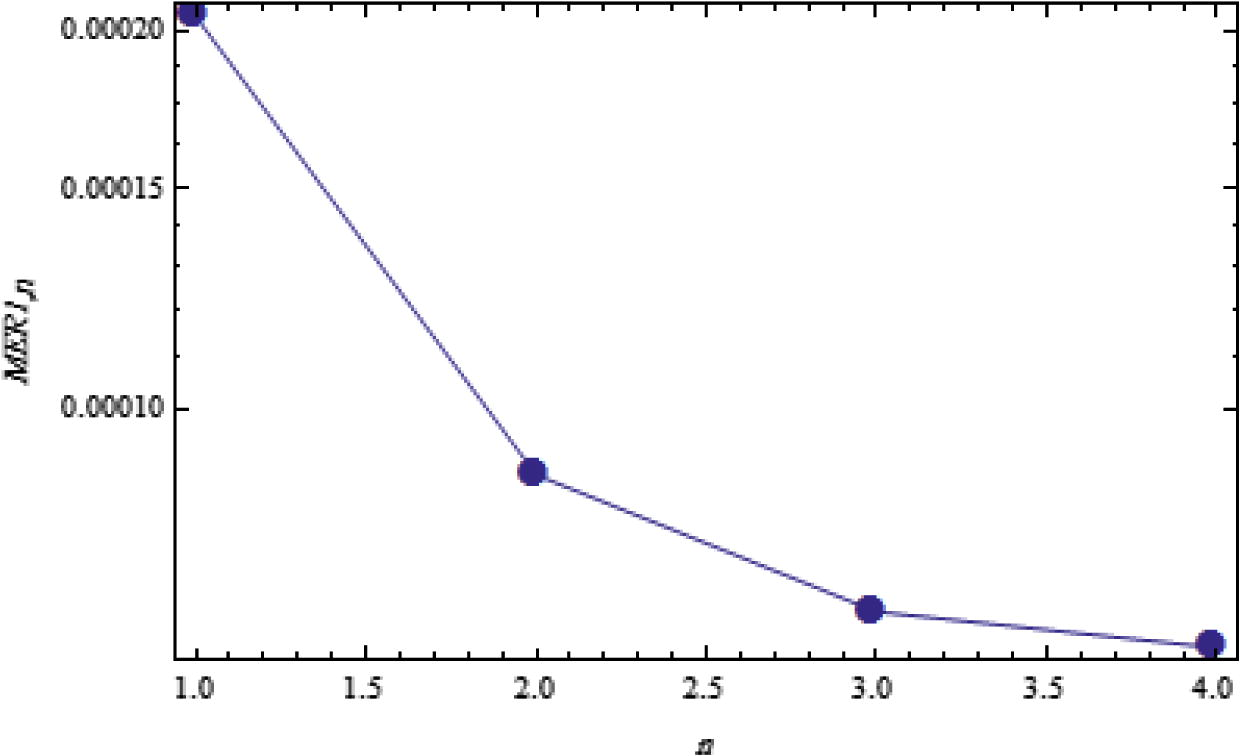
Logarithmic plots of MER1,n against n is 1 through 4 and m = 1.

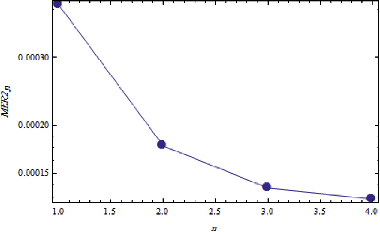
Logarithmic plots of MER2,n against n is 1 through 4 and m = 1.

It is necessary to mention here, the accuracy will be increasing by increase of the denominator of the initial conditions $(\frac{x}{m})$ also the error will be decreasing. Moreover, we can note that as shown in Tables 4 and 5 and Figs. 3 and 4, when we increase the iteration $(n$ from 1 to 4) we obtain a best accuracy. It can be clearly seen that the points lay on straight lines which means an exponential rate of convergence is achieved (see Table 6).

Table 4 Comparison between the ADM, the VIM and TAM of

{MER}_{2, n}

$n$	${MER}_{2, n}$ by the ADM	${MER}_{2, n}$ by the VIM	${MER}_{2, n}$ by the TAM
1	0.0527803	0.00571131	0.000411307
2	0.00636405	0.00228414	0.000176919
3	0.000592835	0.000913568	0.000137548
4	0.000041189	0.000365417	0.000128704

Table 5 The MER_1,n by the TAM, where n = 1,…,4 and x are divided by m.

m	n
m	1	2	3	4
3	$0.000205654$	$0.0000884596$	$0.000068774$	$0.000064352$
5	$0.0000471627$	$0.0000125072$	$5.87609 \times 10^{- 6}$	$3.3354 \times 10^{- 6}$
10	$6.1817 \times 10^{- 6}$	$8.3866 \times 10^{- 7}$	$1.99081 \times 10^{- 7}$	$5.69789 \times 10^{- 8}$
15	$1.86177 \times 10^{- 6}$	$1.69779 \times 10^{- 7}$	$2.69968 \times 10^{- 8}$	$5.16875 \times 10^{- 9}$
20	$7.91955 \times 10^{- 7}$	$5.43946 \times 10^{- 8}$	$6.50441 \times 10^{- 9}$	$9.35771 \times 10^{- 10}$
25	$4.07511 \times 10^{- 7}$	$2.24494 \times 10^{- 8}$	$2.15122 \times 10^{- 9}$	$2.47894 \times 10^{- 10}$
30	$2.36618 \times 10^{- 7}$	$1.08814 \times 10^{- 8}$	$8.69954 \times 10^{- 10}$	$8.36112 \times 10^{- 11}$
35	$1.49365 \times 10^{- 7}$	$5.89497 \times 10^{- 9}$	$4.04314 \times 10^{- 10}$	$3.33282 \times 10^{- 11}$
40	$1.00243 \times 10^{- 7}$	$3.46501 \times 10^{- 9}$	$2.08082 \times 10^{- 10}$	$1.50156 \times 10^{- 11}$
45	$7.05026 \times 10^{- 8}$	$2.16782 \times 10^{- 9}$	$1.15778 \times 10^{- 10}$	$7.42927 \times 10^{- 12}$
50	$5.14541 \times 10^{- 8}$	$1.42474 \times 10^{- 9}$	$6.85117 \times 10^{- 11}$	$3.95786 \times 10^{- 12}$

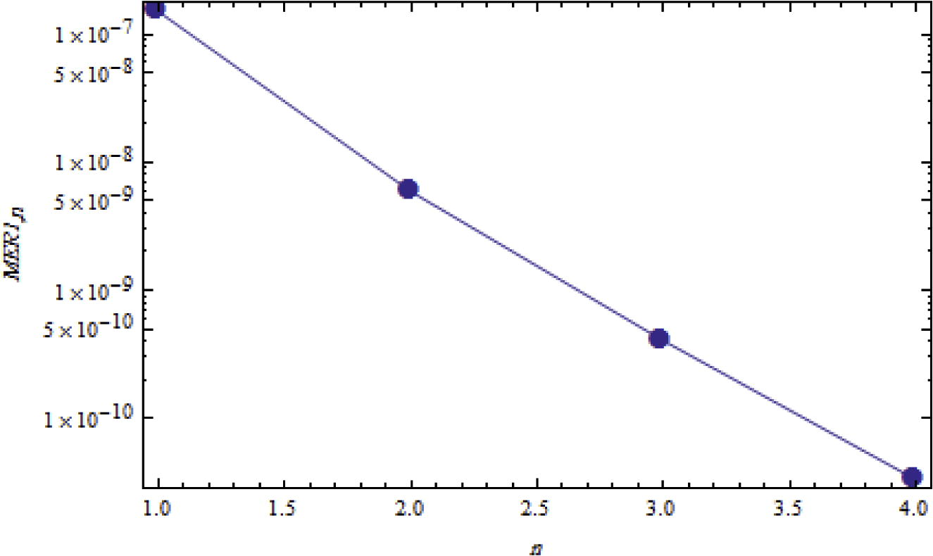
Logarithmic plots of MER1,n against n is 1 through 4 and m = 35.

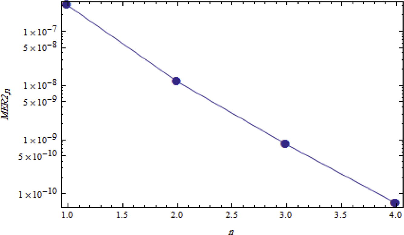
Logarithmic plots of MER2, against n is 1 through 4 and m = 35.

Table 6 The MER_2,n by the TAM where n = 1,…,4 and x are divided by m.

m	n
m	1	2	3	4
3	$0.000411307$	$0.000176919$	$0.000137548$	$0.000128704$
5	$0.0000943255$	$0.0000250144$	$0.0000117522$	$6.6708 \times 10^{- 6}$
10	$0.0000123634$	$1.67732 \times 10^{- 6}$	$3.98162 \times 10^{- 7}$	$1.13958 \times 10^{- 7}$
15	$3.72354 \times 10^{- 6}$	$3.39557 \times 10^{- 7}$	$5.39935 \times 10^{- 8}$	$1.03375 \times 10^{- 8}$
20	$1.58391 \times 10^{- 6}$	$1.08789 \times 10^{- 7}$	$1.30088 \times 10^{- 8}$	$1.87154 \times 10^{- 9}$
25	$8.15022 \times 10^{- 7}$	$4.48988 \times 10^{- 8}$	$4.30245 \times 10^{- 9}$	$4.95789 \times 10^{- 10}$
30	$4.73236 \times 10^{- 7}$	$2.17629 \times 10^{- 8}$	$1.73991 \times 10^{- 9}$	$1.67222 \times 10^{- 10}$
35	$2.98729 \times 10^{- 7}$	$1.17899 \times 10^{- 8}$	$8.08628 \times 10^{- 10}$	$6.66563 \times 10^{- 11}$
40	$2.00486 \times 10^{- 7}$	$6.93002 \times 10^{- 9}$	$4.16165 \times 10^{- 10}$	$3.00313 \times 10^{- 11}$
45	$1.41005 \times 10^{- 7}$	$4.33564 \times 10^{- 9}$	$2.31556 \times 10^{- 10}$	$1.48585 \times 10^{- 11}$
50	$1.02908 \times 10^{- 7}$	$2.84949 \times 10^{- 9}$	$1.37023 \times 10^{- 10}$	$7.91572 \times 10^{- 12}$

7.2

7.2 Numerical simulations of the system of chemical kinetics

In this section, we also compute the error remainders and the maximal error remainders $({MER}_{1, n})$ , $({MER}_{2, n})$ and ${MER}_{3, n}$ to assess the convergence of TAM for the system of chemical kinetics problems. We suppose the values of the three reaction rates are: $c_{1} = 0.1$ , $c_{2} = 0.02$ and $c_{3} = 0.009$ , as given in Aminikhah (2011).

In Tables 7–9 below, the values of ${MER}_{1, n}$ , ${MER}_{2, n}$ and ${MER}_{3, n}$ which are obtained by TAM are compared with those resulted by VIM and HPM (Aminikhah, 2011; Ganji et al., 2007). The results demonstrate that the method has many merits such as, overcoming the difficulty arising in calculating Adomian polynomials to handle the nonlinear terms in ADM. It does not require to calculate Lagrange multiplier as in VIM (which is time consuming) and does not need to construct a homotopy and solve the corresponding algebraic equations as in HPM.

Table 7 Comparison between the HPM, the VIM and TAM of MER_1,n.

$n$	${MER}_{1, n}$ by the HPM	${\begin{matrix} MER \end{matrix}}_{1, n}$ by the VIM	${MER}_{1, n}$ by the TAM
1	$0.001$	$0.001$	$0.001$
2	$5 . \times 10^{- 6}$	$4.99999 \times 10^{- 6}$	$4.99999 \times 10^{- 6}$
3	$1.66726 \times 10^{- 8}$	$1.66666 \times 10^{- 8}$	$1.66666 \times 10^{- 8}$
4	$3.57414 \times 10^{- 11}$	$4.16664 \times 10^{- 11}$	$4.16665 \times 10^{- 11}$

Table 8 Comparison between the ADM, the VIM and TAM of MER_2,n.

$n$	${MER}_{2, n}$ by the HPM	${MER}_{2, n}$ by the VIM	${MER}_{2, n}$ by the TAM
1	$0.0010009$	$0.0010009$	$0.0010009$
2	$4.10898 \times 10^{- 6}$	$5.00898 \times 10^{- 6}$	$5.00898 \times 10^{- 6}$
3	$7.71961 \times 10^{- 9}$	$1.66965 \times 10^{- 8}$	$1.66965 \times 10^{- 8}$
4	$1.12015 \times 10^{- 11}$	$4.17412 \times 10^{- 11}$	$4.17412 \times 10^{- 11}$

Table 9 Comparison between the ADM, the VIM and TAM of MER_3,n.

$n$	${MER}_{3, n}$ by the HPM	${MER}_{3, n}$ by the VIM	${MER}_{3, n}$ by the TAM
1	$9 . \times 10^{- 7}$	$9 . \times 10^{- 7}$	$9 . \times 10^{- 7}$
2	$8.91023 \times 10^{- 7}$	$8.98287 \times 10^{- 9}$	$8.98287 \times 10^{- 9}$
3	$8.95302 \times 10^{- 9}$	$2.98904 \times 10^{- 11}$	$2.98904 \times 10^{- 11}$
4	$4.69428 \times 10^{- 11}$	$7.4733 \times 10^{- 14}$	$7.4733 \times 10^{- 14}$

We can note that in Tables 7–9 below, the increase in the values of $n$ from 1 to 4 leads to the decrease in the values of ${MER}_{1, n}$ , ${MER}_{2, n}$ and ${MER}_{3, n}$ as follows:

Furthermore, we can show the analysis of the maximal error remainders for MER_1,n, MER_2,n and MER_3,n, respectively, through the Figs. 5–7 , where the points lay on a straight line which means we achieved an exponential rate of convergence.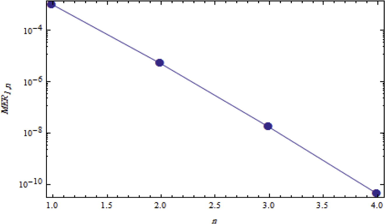

Logarithmic plots of MER1,n against n is 1 through 4.

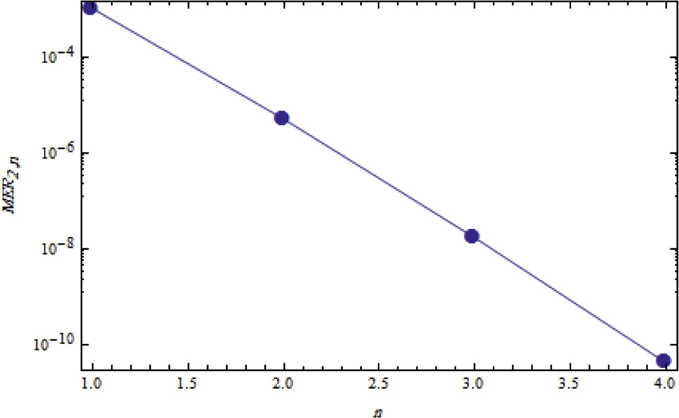
Logarithmic plots of MER2,n against n is 1 through 4.

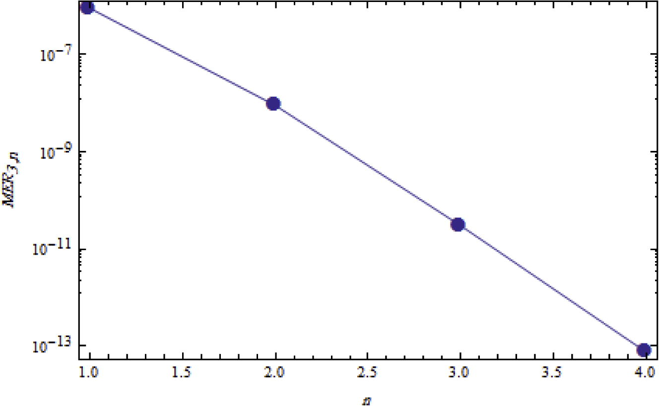
Logarithmic plots of MER3,n against n is 1 through 4.

8 Conclusion

In the present paper, the semi-analytical iterative technique (TAM) is implemented for solving the two systems of chemical problems which are represented by systems of nonlinear ordinary differential equations. We have presented the convergence and accuracy of the method (TAM) for the systems of nonlinear equations by theorems and numerical results. Through the figures and tables, it can be seen clearly that the maximal error remainders decreased when the number of iterations are increased. Numerical results showed that for both systems of chemical problems the TAM is able to generate accurate solutions with exponential rate of the convergence. Motivation of current work is achieved by comparing the Runge–Kutta method (RK4) with TAM for an example in which the exact solution is available. Numerical experiments demonstrated that the suggested method possesses the high-order accuracy in comparison of RK4 with some other existing technique. Also, the main goal of the current paper is achieved by solving the two systems of chemical problems accurately with reliable results.

Furthermore, in comparison with the some existing methods such as ADM, HPM and VIM results, it is observed in general that the approximate solutions obtained by the TAM converge faster without any restricted assumptions.

Acknowledgements

The author would like to thank the anonymous referees and Editor-in-Chief for their valuable suggestions.

References

AL-Jawary M.A., Radhi G.H., . The Variational Iteration Method for calculating carbon dioxide absorbed into phenyl glycidyl ether. IOSR J. Math.. 2015;11:99-105.
[Google Scholar]
AL-Jawary M.A., Raham R.K., Radhi G.H., . An iterative method for calculating carbon dioxide absorbed into phenyl glycidyl ether. J. Math. Comput. Sci.. 2016;6(4):620-632.
[Google Scholar]
Aminikhah H., . An analytical approximation to the solution of chemical kinetics system. J. King Saud Univ. Sci.. 2011;23:167-170.
[Google Scholar]
Bellman R.E., Kalaba R.E., . Quasi linearisation and nonlinear boundary-value problems. New York: Elsevier; 1965.
Bildik N., Deniz S., . Implementation of Taylor collocation and Adomian decomposition method for systems of ordinary differential equations. AIP Conf. Proc.. 2015;1648:370002.
[CrossRef] [Google Scholar]
Bildik N., Deniz S., . Comparison of solutions of systems of delay differential equations using Taylor collocation method, lambert w function and variational iteration method. Sci. Iran. Trans. D Comput. Sci. Eng. Electr.. 2015;22:1-15.
[Google Scholar]
Cá zares-Ramı́rez R.-I., Espinosa-Paredes G., . Time-fractional telegraph equation for hydrogen diffusion during severe accident in BWRs. J. King Saud Univ. Sci.. 2016;28:21-28.
[Google Scholar]
Choe Y.S., Oh K.J., Kim M.C., Park S.W., . Chemical absorption of carbon dioxide into phenyl lycidyl ether solution containing THA–CP–MS41 catalyst. Korean J. Chem. Eng.. 2010;27:1868-1875.
[Google Scholar]
Deniz S., Bildik N., . Comparison of adomian decomposition method and Taylor matrix method in solving different kinds of partial differential equations. Int. J. Model. Optim.. 2014;4:292-298.
[Google Scholar]
Duan J., Rach R., Wazwaz A.M., . Steady-state concentrations of carbon dioxide absorbed into phenyl glycidyl ether solutions by the Adomian decomposition method. J. Math. Chem.. 2015;53:1054-1067.
[Google Scholar]
Ehsani F., Hadi A., Ehsani F., Mahdavi R., . An iterative method for solving partial differential equations and solution of Korteweg-de Vries equations for showing the capability of the iterative method. World Appl. Program.. 2013;3(8):320-327.
[Google Scholar]
El-Zahar E.R., . Approximate analytical solutions of singularly perturbed fourth order boundary value problems using differential transform method. J. King Saud Univ. Sci.. 2013;25:257-265.
[Google Scholar]
Ganji D.D., . A semi-analytical technique for non-linear settling particle equation of motion. J. Hydro-environ. Res.. 2012;6:323-327.
[Google Scholar]
Ganji D.D., Rafei M., . Solitary wave solutions for generalized Hirota-Satsuma coupled KdV equation by homotopy perturbation method. Phys. Lett. A. 2006;356:131-137.
[Google Scholar]
Ganji D.D., Nourollahi M., Mohseni E., . Application of He’s methods to nonlinear chemistry problems. Comput. Math. Appl.. 2007;54:112-1132.
[Google Scholar]
Jerri A., . Introduction to Integral Equation with Applications. Marcel Dekker; 1985.
Khader M.M., . On the numerical solutions for chemical kinetics system using picard-pade technique. J. King Saud Univ. Sci.. 2013;25:97-103.
[Google Scholar]
Makinde O.D., . Adomian decomposition approach to a SIR epidemic model with constant vaccination strategy. Appl. Math. Comput.. 2007;184:842-848.
[Google Scholar]
Makinde O.D., . Solving ratio-dependent predator-prey system with constant effort harvesting using Adomian decomposition method. Appl. Math. Comput.. 2007;186:17-22.
[Google Scholar]
Makinde O.D., . On non-perturbative approach to transmission dynamics of infectious diseases with waning immunity. Int. J. Nonlinear Sci. Numer. Simul.. 2009;10:451-458.
[Google Scholar]
Matinfar M., Saiedy M., Gharahsulfu B., Eslami M., . Solutions of nonlinear chemistry problems by homotopy analysis method. Comput. Math. Model.. 2014;25(1):103-114.
[Google Scholar]
Matinfar M., Mirzanezhad S., Ghasemi M., Salehi M., . Solving the interaction of electromagnetic wave with electron by VIM. J. King Saud Univ. Sci.. 2015;27:63-70.
[Google Scholar]
Muthukaruppan S., Krishnaperumal I., Lakshmanan R., . Theoretical analysis of mass transfer with chemical reaction using absorption of carbon dioxide into phenyl glycidyl ether solution. Appl. Math.. 2012;3:1179-1186.
[Google Scholar]
Saadatmandi A., Dehghan M., Eftekhari A., . Application of He’s homotopy perturbation method for nonlinear system of second-order boundary value problems. Nonlinear Anal.: Real World Appl.. 2009;10:1912-1922.
[Google Scholar]
Temimi H., Ansari A.R., . A semi – analytical iterative technique for solving nonlinear problems. Comput. Math. Appl.. 2011;61:203-210.
[Google Scholar]
Temimi H., Ansari A.R., . A new iterative technique for solving nonlinear second order multi – point boundary value problems. Appl. Math. Comput.. 2011;218:1457-1466.
[Google Scholar]
Temimi H., Ansari A.R., . A computational iterative method for solving nonlinear ordinary differential equations. LMS J. Comput. Math.. 2015;18:730-753.
[Google Scholar]
Vazquez-Leal H., Rashidinia J., Hernandez-Martinez L., Daei-Kasmaei H., . A comparison of HPM, NDHPM, Picard and Picard–Padé methods for solving Michaelis-Menten equation. J. King Saud Univ. Sci.. 2015;27:7-14.
[Google Scholar]
Wazwaz A.M., . Adomian decomposition method for a reliable treatment of the Bratu-type equations. Appl. Math. Comput.. 2005;166:652-663.
[Google Scholar]

Appendix A

MATHEMATICA code for applying the RK4 for the system given in Eq. (51)

ClearAll[“Global‘ *”] $ClassicalRungeKuttaCoefficients [4,prec_] : = With [{amat = {{1 / 2}, {0, 1 / 2}, {0, 0, 1}},bvec = {1 / 6, 1 / 3, 1 / 3, 1 / 6},cvec = {1 / 2, 1 / 2, 1}}, N [{amat,bvec,cvec},prec]]$ ${w 1 f,w 2 f} = {w 1, w 2} / . First @ NDSolve [{w 1^{″} [t] = = t * w 2^{'} [t] - w 1 [t] + t^{3} - 2 * t^{2} + 6 * t, w 2^{″} [t] = = - t * w 1^{'} [t] - w 1 [t] * w 2 [t] + t^{5} - t^{4} + 2 * t^{3} + t^{2} - t + 2, w 1 [0] = = 0, w 1 [1] = = 0, w 2 [0] = = 0, w 2 [1] = = 0}, {w 1, w 2}, {t, 0, 0.1},Method \to {“ Explicit Runge Kutta ”, “ DifferenceOrder ” \to 4, “ Coefficients ” \to Classical Runge Kutta Coefficients},Starting Step Size \to 0.01];$ $wlff = MapThread [Append, {w 1 f [“ Grid ”],w 1 f [“ ValuesOnGrid ”]}]$ $w 2 ff = MapThread [Append, {w 2 f [“ Grid ”],w 2 f [“ ValuesOnGrid ”]}]$

Show Sections

[1] AL-Jawary M.A., Radhi G.H., . The Variational Iteration Method for calculating carbon dioxide absorbed into phenyl glycidyl ether. IOSR J. Math.. 2015;11:99-105.
[Google Scholar]

[2] AL-Jawary M.A., Raham R.K., Radhi G.H., . An iterative method for calculating carbon dioxide absorbed into phenyl glycidyl ether. J. Math. Comput. Sci.. 2016;6(4):620-632.
[Google Scholar]

[3] Aminikhah H., . An analytical approximation to the solution of chemical kinetics system. J. King Saud Univ. Sci.. 2011;23:167-170.
[Google Scholar]

[4] Bellman R.E., Kalaba R.E., . Quasi linearisation and nonlinear boundary-value problems. New York: Elsevier; 1965.

[5] Bildik N., Deniz S., . Implementation of Taylor collocation and Adomian decomposition method for systems of ordinary differential equations. AIP Conf. Proc.. 2015;1648:370002.
[CrossRef] [Google Scholar]

[6] Bildik N., Deniz S., . Comparison of solutions of systems of delay differential equations using Taylor collocation method, lambert w function and variational iteration method. Sci. Iran. Trans. D Comput. Sci. Eng. Electr.. 2015;22:1-15.
[Google Scholar]

[7] Cá zares-Ramı́rez R.-I., Espinosa-Paredes G., . Time-fractional telegraph equation for hydrogen diffusion during severe accident in BWRs. J. King Saud Univ. Sci.. 2016;28:21-28.
[Google Scholar]

[8] Choe Y.S., Oh K.J., Kim M.C., Park S.W., . Chemical absorption of carbon dioxide into phenyl lycidyl ether solution containing THA–CP–MS41 catalyst. Korean J. Chem. Eng.. 2010;27:1868-1875.
[Google Scholar]

[9] Deniz S., Bildik N., . Comparison of adomian decomposition method and Taylor matrix method in solving different kinds of partial differential equations. Int. J. Model. Optim.. 2014;4:292-298.
[Google Scholar]

[10] Duan J., Rach R., Wazwaz A.M., . Steady-state concentrations of carbon dioxide absorbed into phenyl glycidyl ether solutions by the Adomian decomposition method. J. Math. Chem.. 2015;53:1054-1067.
[Google Scholar]

[11] Ehsani F., Hadi A., Ehsani F., Mahdavi R., . An iterative method for solving partial differential equations and solution of Korteweg-de Vries equations for showing the capability of the iterative method. World Appl. Program.. 2013;3(8):320-327.
[Google Scholar]

[12] El-Zahar E.R., . Approximate analytical solutions of singularly perturbed fourth order boundary value problems using differential transform method. J. King Saud Univ. Sci.. 2013;25:257-265.
[Google Scholar]

[13] Ganji D.D., . A semi-analytical technique for non-linear settling particle equation of motion. J. Hydro-environ. Res.. 2012;6:323-327.
[Google Scholar]

[14] Ganji D.D., Rafei M., . Solitary wave solutions for generalized Hirota-Satsuma coupled KdV equation by homotopy perturbation method. Phys. Lett. A. 2006;356:131-137.
[Google Scholar]

[15] Ganji D.D., Nourollahi M., Mohseni E., . Application of He’s methods to nonlinear chemistry problems. Comput. Math. Appl.. 2007;54:112-1132.
[Google Scholar]

[16] Jerri A., . Introduction to Integral Equation with Applications. Marcel Dekker; 1985.

[17] Khader M.M., . On the numerical solutions for chemical kinetics system using picard-pade technique. J. King Saud Univ. Sci.. 2013;25:97-103.
[Google Scholar]

[18] Makinde O.D., . Adomian decomposition approach to a SIR epidemic model with constant vaccination strategy. Appl. Math. Comput.. 2007;184:842-848.
[Google Scholar]

[19] Makinde O.D., . Solving ratio-dependent predator-prey system with constant effort harvesting using Adomian decomposition method. Appl. Math. Comput.. 2007;186:17-22.
[Google Scholar]

[20] Makinde O.D., . On non-perturbative approach to transmission dynamics of infectious diseases with waning immunity. Int. J. Nonlinear Sci. Numer. Simul.. 2009;10:451-458.
[Google Scholar]

[21] Matinfar M., Saiedy M., Gharahsulfu B., Eslami M., . Solutions of nonlinear chemistry problems by homotopy analysis method. Comput. Math. Model.. 2014;25(1):103-114.
[Google Scholar]

[22] Matinfar M., Mirzanezhad S., Ghasemi M., Salehi M., . Solving the interaction of electromagnetic wave with electron by VIM. J. King Saud Univ. Sci.. 2015;27:63-70.
[Google Scholar]

[23] Muthukaruppan S., Krishnaperumal I., Lakshmanan R., . Theoretical analysis of mass transfer with chemical reaction using absorption of carbon dioxide into phenyl glycidyl ether solution. Appl. Math.. 2012;3:1179-1186.
[Google Scholar]

[24] Saadatmandi A., Dehghan M., Eftekhari A., . Application of He’s homotopy perturbation method for nonlinear system of second-order boundary value problems. Nonlinear Anal.: Real World Appl.. 2009;10:1912-1922.
[Google Scholar]

[25] Temimi H., Ansari A.R., . A semi – analytical iterative technique for solving nonlinear problems. Comput. Math. Appl.. 2011;61:203-210.
[Google Scholar]

[26] Temimi H., Ansari A.R., . A new iterative technique for solving nonlinear second order multi – point boundary value problems. Appl. Math. Comput.. 2011;218:1457-1466.
[Google Scholar]

[27] Temimi H., Ansari A.R., . A computational iterative method for solving nonlinear ordinary differential equations. LMS J. Comput. Math.. 2015;18:730-753.
[Google Scholar]

[28] Vazquez-Leal H., Rashidinia J., Hernandez-Martinez L., Daei-Kasmaei H., . A comparison of HPM, NDHPM, Picard and Picard–Padé methods for solving Michaelis-Menten equation. J. King Saud Univ. Sci.. 2015;27:7-14.
[Google Scholar]

[29] Wazwaz A.M., . Adomian decomposition method for a reliable treatment of the Bratu-type equations. Appl. Math. Comput.. 2005;166:652-663.
[Google Scholar]

A semi-analytical iterative technique for solving chemistry problems

Abstract

Keywords

Chemical problems

Systems of ordinary differential equations

Approximate solutions

The maximal error remainders

1 Introduction

2 Steady-state of the chemical problems

2.1 Condensations of carbon dioxide and phenyl glycidyl ether

2.2 Chemical kinetics problem

3 Basic idea of semi-analytical iterative technique (TAM)

4 Solving the chemical problems by TAM

4.1 Problem (1)

4.2 Problem (2)

5 Convergence and error analysis

6 Convergence of initial value problems

7 Numerical simulations

7.1 Numerical simulations of the system of condensations of CO2 and PGE

7.2 Numerical simulations of the system of chemical kinetics

8 Conclusion

Acknowledgements

References

Appendix A

MATHEMATICA code for applying the RK4 for the system given in Eq. (51)

7.1 Numerical simulations of the system of condensations of CO₂ and PGE