A non-linear study of optical solitons for Kaup-Newell equation without four-wave mixing

Hamood Ur Rehman; Aziz Ullah Awan; Kashif Ali Abro; ElSayed M. Tag El Din; Sobia Jafar; Ahmed M. Galal

doi:10.1016/j.jksus.2022.102056

View/Download PDF

Buy Reprints

PDF

Translate this page into:

Original article

07 2022

:34;

102056

doi:

10.1016/j.jksus.2022.102056

A non-linear study of optical solitons for Kaup-Newell equation without four-wave mixing

Hamood Ur Rehman^{^a}, Aziz Ullah Awan^{^b}, Kashif Ali Abro^{^c,^d,⁎}, ElSayed M. Tag El Din^{^e}, Sobia Jafar^{^a}, Ahmed M. Galal^{^f,^g}

a Department of Mathematics, University of Okara, Okara, Pakistan

b Department of Mathematics, University of the Punjab, Lahore, Pakistan

c Institute of Ground Water Studies, Faculty of Natural and Agricultural Sciences, University of the Free State, Bloemfontein, South Africa

d Department of Basic Sciences and Related Studies, Mehran University of Engineering and Technology, Jamshoro, Pakistan

e Electrical Engineering Department, Faculty of Engineering & Technology, Future University in Egypt New Cairo 11835, Egypt

f Mechanical Engineering Department, College of Engineering, Prince Sattam Bin Abdulaziz University, Wadi addawaser11991, Saudi Arabia

g Production Engineering and Mechanical Design Department, Faculty of Engineering, Mansoura University, P.O 35516, Mansoura, Egypt

⁎Corresponding author at: Institute of Ground Water Studies, Faculty of Natural and Agricultural Sciences, University of the Free State, Bloemfontein, South Africa. kashif.abro@faculty.muet.edu.pk (Kashif Ali Abro)

Received: 2020-11-29, Accepted: 2022-4-22,

Disclaimer:
This article was originally published by Elsevier and was migrated to Scientific Scholar after the change of Publisher.

Peer review under responsibility of King Saud University.

Abstract

Nonlinear science is a fundamental science frontier that include studies and the common properties of nonlinear phenomena. This article is devoted to the study of sub-pico second optical pluses in birefringent fibers for Kaup-Newell equation (KNE) without four-wave mixing. Three prominent integrations techniques are successfully implemented on KNE in coupled vector form. Variety of soliton solutions namely dark, bright, periodic singular, singular and bright-singular combo solitons are constructed for the KNE in birefringent fibers. The obtained solutions are reckoned with their respective existence criterion. In addition, two-dimensional and three-dimensional graphs are drawn to exhibit the physical behavior of the obtained solutions.

Keywords

Nonlinear

Birefringent fibers

Optical solitons

Kaup-Newell Equation

Four-Wave Mixing

Show Related Articles from PubMed

1 Introduction

Nonlinear PDEs frequently appears in basic laws of nature. In the mathematical physics and other domains of applied sciences, several models obviously arise from solid state physics, plasma physics, ocean hydrodynamics, atmospheric waves, biology, chemistry, mathematical materials sciences, etc (Abbagari et al., 2021; An et al., 2020; Awan et al., 2021; Hosseini et al., 2019; Rehman et al., 2020; Shahen et al., 2020; Tahir and Awan, 2019; Tahir and Awan, 2020; Yepez-Martinez et al., 2018; Yoku et al., 2020 ). Witout deep understanding of soliton dynamic the modern technology considered to be impossible. The working communication channel such as internet, facebook, cell phones, electronic mail and twitter depend on soliton propagation.

In recent years, the area of soliton propagation in nonlinear optical media have testified a lot of research. These researches have current applications on communication technology reliant on the transmission of optical local pulses. The optical soliton solution is the dynamic area of recent science especially in nonlinear optics. A large number of methods are introduced and applied to find optical soliton solution such as Kudryashov’s method, first integral technique, mapping technique, $(G^{'} / G)$ -expansion technique, undetermined coefficient method, functional variable method, generalized Kudryashov’s method, modified simple equation method, new extended direct algebraic method and many others (Delgado et al., 2018; Ghanbari and Aguilar, 2019; Martinez et al., 2018; Morales-Delgado et al., 2018; Rehman et al., 2019; Rehman et al., 2019; Rehman et al., 2019; Sedeeg et al., 2019; Tahir et al., 2019 ).

The KNE (Arshed et al., 2018; Biswas et al., 2018; Biswas et al., 2018; Jawad et al., 2019; Triki et al., 2019 ) is taken a most popular form of the NLSE. This model is useful to explain the propagation of modulated structures in plasma physics and optical fiber especially Alfven waves.

In this article, we study the nonlinear KNE in birefringent fiber without four-wave mixing (FWM) (Ahmed et al., 2020; Yildirim et al., 2019). FWM expresses a nonlinear optical effect in which four waves interact each other as a result of the third order nonlinearity. There are numerous mathematical analysis to study the NLEEs in birefringent fibers (Awan et al., 2020; Bhrawy et al., 2014; Rehman et al., 2020; Rehman et al., 2020; Rehman et al., 2020; Tahir and Awan, 2020; Tahir et al., 2019 ). The optical soliton solutions of KNE in birefringent fibers are not much studied in the previous literature. Here, three different techniques namely Kudryashov’s method (Rehman et al., 2019; Rehman et al., 2019), undetermined coefficient method (Morales-Delgado et al., 2018; Sedeeg et al., 2019) and modified mapping method (Rehman et al., 2019; Rehman et al., 2020) are adopted to extract solutions of KNE in birefringent without FWM. In this context, the we adhere few recent attempts on analytical as well as numerical approaches of dynamical mathematical models as well (Arshad et al., 2017; Liu et al., 2020; Hosseini et al., 2021; Hussain et al., 2021; Memon et al., 2020; Syed et al., 2021 ). These integration algorithms are successfully applied to extract dark, bright, singular, bright-singular and periodic singular combo soliton solutions.

The KNE polarization-preserving fibers (An et al., 2020; Hosseini et al., 2019; Rehman et al., 2020; Shahen et al., 2020 ) is given as

(1)

p_{t} + ι {ap}_{xx} + b {(| p |^{2} p)}_{x} = 0 .

In the model (1), a and b are the coefficients of GVD and the nonlinearity respectively. The KNE in coupled vector form without FWM reads

(2)

\begin{matrix} ϕ_{t} + ι a_{1} ϕ_{xx} + λ_{1} {(| ϕ |^{2} ϕ)}_{x} + γ_{1} {(| ψ |^{2} ψ)}_{x} = 0, \\ ψ_{t} + ι a_{2} ψ_{xx} + λ_{2} {(| ψ |^{2} ψ)}_{x} + γ_{2} {(| ϕ |^{2} ϕ)}_{x} = 0 . \end{matrix}

The constants $a_{i}, λ_{i}$ and $γ_{i}$ assure the GVD and nonlinearity.

2 Mathematical Analysis

To solve system of Eqs. (2), we substitute

(3)

\begin{matrix} ϕ (x, t) = Q_{1} (ϑ) e^{ι φ (x, t)}, \\ ψ (x, t) = Q_{2} (ϑ) e^{ι φ (x, t)} . \end{matrix}

Here $Q_{i} (ϑ)$ represents amplitude, where

(4)

ϑ = x - η t, φ (x, t) = θ_{0} + ω t - kx,

where

k, η, ω

and

θ_{0}

sequentially represent frequency, velocity, wave number and phase constant.

By substituting $(3)$ into $(2)$ and then the real and imaginary parts are respectively given as

(5)

(2 {ka}_{i} - η) Q'_{i} + 3 λ_{i} Q'_{i} Q_{i}^{2} + 3 γ_{i} Q'_{\tilde{i}} Q_{\tilde{i}}^{2} = 0,

(6)

a_{i} Q''_{i} - (a_{i} k^{2} - ω) Q_{i} - k λ_{i} Q_{i}^{3} - k γ_{i} Q_{\tilde{i}}^{3} = 0 .

By using the balancing condition $Q_{i} = Q_{\tilde{i}}$ , then the real and imaginary parts emerged as

(7)

Q_{i} (2 {ka}_{i} - η) + Q_{i}^{3} (λ_{i} + γ_{i}) = 0,

(8)

a_{i} Q''_{i} - Q_{i} (a_{i} k^{2} - ω) - Q_{i}^{3} k (λ_{i} + γ_{i}) = 0 .

Eq. (7) gives the soliton velocity as

(9)

η = 2 {ka}_{i} + Q_{i}^{2} (λ_{i} + γ_{i}) .

In the next subsections, Eq. (8) is solved using the above mentioned integration methods.

2.1

2.1 Bright Soliton

Let the solution of $(8)$ in form of bright soliton is taken as

(10)

Q_{i} (ϑ) = {Asech}^{r} (B ϑ), ϑ = x - η t .

Setting (10) into (8), we have

(11)

- r (r + 1) a_{i} {AB}^{2} {sech}^{r + 2} (B ϑ) + {Asech}^{r} (B ϑ) [ω - a_{i} k^{2} + a_{i} r^{2} B^{2}] - A^{3} {sech}^{3 r} (B ϑ) (λ_{i} + γ_{i}) k = 0 .

By balancing, we get $r = 1$ , comparing the coefficients of linearly independent terms give

(12)

A = \pm \sqrt{- \frac{2 (a_{i} k^{2} - ω)}{k (λ_{i} + γ_{i})}}, B = \pm \sqrt{\frac{a_{i} k^{2} - ω}{a_{i}}} .

(13)

Q_{i} (ϑ) = \pm \sqrt{- \frac{2 (a_{i} k^{2} - ω)}{k (λ_{i} + γ_{i})}} sech (\sqrt{\frac{a_{i} k^{2} - ω}{a_{i}}} (x - η t)) .

Substituting (13) into (3), we obtain the bright soliton solutions as

(14)

ϕ (x, t) = \pm \sqrt{- \frac{2 (a_{1} k^{2} - ω)}{k (λ_{1} + γ_{1})}} sech (\sqrt{\frac{a_{1} k^{2} - ω}{a_{1}}} (x - η t)) e^{ι (- kx + ω t + θ_{0})},

and

(15)

ψ (x, t) = \pm \sqrt{- \frac{2 (a_{2} k^{2} - ω)}{k (λ_{2} + γ_{2})}} sech (\sqrt{\frac{a_{2} k^{2} - ω}{a_{2}}} (x - η t)) e^{ι (- kx + ω t + θ_{0})} .

2.2

2.2 Dark Soliton

The dark soliton of $(8)$ is taken as

(16)

Q_{i} (ϑ) = {Atanh}^{r} (B ϑ) .

Setting (16) into (8), we have

(17)

\begin{matrix} r (r - 1) a_{i} {AB}^{2} \tanh^{r - 2} (B ϑ) + {Atanh}^{r} (B ϑ) [ω - a_{i} k^{2} - 2 a_{i} r^{2} B^{2}] + \\ r (r + 1) a_{i} {AB}^{2} \tanh^{r + 2} (B ϑ) - A^{3} \tanh^{3 r} (B ϑ) (λ_{i} + γ_{i}) k = 0 . \end{matrix}

By balancing we get $r = 1$ and then comparing the coefficients of linearly independent terms give

(18)

A = \pm \sqrt{- \frac{a_{i} k^{2} - ω}{k (λ_{i} + γ_{i})}}, B = \pm \sqrt{- \frac{a_{i} k^{2} - ω}{2 a_{i}}} .

(19)

Q_{i} (ϑ) = \pm \sqrt{- \frac{a_{i} k^{2} - ω}{k (λ_{i} + γ_{i})}} \tanh (\sqrt{- \frac{a_{i} k^{2} - ω}{2 a_{i}}} (x - η t)) .

Substituting (19) into (3), we obtain solutions in the form of dark soliton as

(20)

ϕ (x, t) = \pm \sqrt{- \frac{a_{1} k^{2} - ω}{k (λ_{1} + γ_{1})}} \tanh (\sqrt{- \frac{a_{1} k^{2} - ω}{2 a_{1}}} (x - η t)) e^{ι (- kx + ω t + θ_{0})},

(21)

ψ (x, t) = \pm \sqrt{- \frac{a_{2} k^{2} - ω}{k (λ_{2} + γ_{2})}} \tanh (\sqrt{- \frac{a_{2} k^{2} - ω}{2 a_{2}}} (x - η t)) e^{ι (- kx + ω t + θ_{0})} .

2.3

2.3 Singular Soliton (Type-I)

Let solution of (8) in the form of singular soliton is taken as

(22)

Q_{i} (ϑ) = {Acsch}^{r} (B ϑ) .

Setting (22) into (8), we have

(23)

r (r + 1) a_{i} {AB}^{2} {csch}^{r + 2} (B ϑ) + {Acsch}^{r} (B ϑ) [ω - a_{i} k^{2} + a_{i} r^{2} B^{2}] - A^{3} {csch}^{3 r} (B ϑ) (λ_{i} + γ_{i}) k = 0 .

By balancing we get $r = 1$ and then comparing the coefficients of linearly independent terms give

(24)

A = \pm \sqrt{\frac{2 (a_{i} k^{2} - ω)}{k (λ_{i} + γ_{i})}}, B = \pm \sqrt{\frac{a_{i} k^{2} - ω}{a_{i}}} .

(25)

Q_{i} (ϑ) = \pm \sqrt{\frac{2 (a_{i} k^{2} - ω)}{k (λ_{i} + γ_{i})}} csch (\sqrt{\frac{a_{i} k^{2} - ω}{a_{i}}} (x - η t)) .

Substituting (25) into (3), we get the singular soliton solutions as

(26)

ϕ (x, t) = \pm \sqrt{\frac{2 (a_{1} k^{2} - ω)}{k (λ_{1} + γ_{1})}} csch (\sqrt{\frac{a_{1} k^{2} - ω}{a_{1}}} (x - η t)) e^{ι (- kx + ω t + θ_{0})},

and

(27)

ψ (x, t) = \pm \sqrt{\frac{2 (a_{2} k^{2} - ω)}{k (λ_{2} + γ_{2})}} csch (\sqrt{\frac{a_{2} k^{2} - ω}{a_{2}}} (x - η t)) e^{ι (- kx + ω t + θ_{0})} .

2.4

2.4 Singular Soliton (Type-II)

The dark soliton of $(8)$ is taken as

(28)

Q_{i} (ϑ) = {Acoth}^{r} (B ϑ) .

Setting (28) into (8), we have

(29)

r (r - 1) a_{i} {AB}^{2} \coth^{r - 2} (B ϑ) + {Acoth}^{r} (B ϑ) [ω - a_{i} k^{2} - 2 a_{i} r^{2} B^{2}] + r (r + 1) a_{i} {AB}^{2} \coth^{r + 2} (B ϑ) - A^{3} \coth^{3 r} (B ϑ) (λ_{i} + γ_{i}) k = 0 .

By balancing, we get $r = 1$ and then comparing the coefficients of linearly independent terms provide the same values as in dark soliton ansatz. So

(30)

Q_{i} (ϑ) = \pm \sqrt{- \frac{a_{i} k^{2} - ω}{k (λ_{i} + γ_{i})}} \coth (\sqrt{- \frac{a_{i} k^{2} - ω}{2 a_{i}}} (x - η t)),

(31)

ϕ (x, t) = \pm \sqrt{- \frac{a_{1} k^{2} - ω}{k (λ_{1} + γ_{1})}} \coth (\sqrt{- \frac{a_{1} k^{2} - ω}{2 a_{1}}} (x - η t)) e^{ι (- kx + ω t + θ_{0})},

(32)

ψ (x, t) = \pm \sqrt{- \frac{a_{2} k^{2} - ω}{k (λ_{2} + γ_{2})}} \coth (\sqrt{- \frac{a_{2} k^{2} - ω}{2 a_{2}}} (x - η t)) e^{ι (- kx + ω t + θ_{0})} .

2.5

2.5 Kudryashov’s Method

Considering the general form of a PDE as

(33)

G (g, g_{t}, g_{x}, g_{tt}, g_{xx}, g_{xt}, \dots .) = 0,

where

g (x, t)

is an unknown function.

Taking following wave transformation

(34)

g (x, t) = Q_{i} (ϑ), ϑ = x - η t,

which converts the above PDE into following ODE

(35)

H (Q_{i}, Q_{i}', Q_{i}'', \dots) = 0 .

According to the Kudryashov’s method, the following finite series states the solution

(36)

Q_{i} (ϑ) = \sum_{j = 0}^{N} c_{j} {(R (ϑ))}^{j},

where

c_{j}

are constants and

R (ϑ)

satisfies

(37)

R (ϑ) = \frac{1}{1 + {de}^{ϑ}} .

Eq. (37) satisfies the following nonlinear differential equation

(38)

\frac{dR}{d ϑ} = R (ϑ) (R (ϑ) - 1) .

Putting (38) into (36), we get algebraic equations in $c_{j}$ by taking the coefficients of powers of $R (ϑ)$ equal to zero.

Thus the solution of Eq. (8) can be expressed as

(39)

Q_{i} = c_{0} + c_{1} R (ϑ),

where

c_{0}

and

c_{1}

are constants. Eq. (8) can be rewritten as

(40)

{AQ}_{i}'' + {BQ}_{i} - k (λ_{i} + γ_{i}) Q_{i}^{3} = 0,

where

(41)

A = a_{1}, B = - (a_{i} k^{2} - ω) .

Substituting (39) into (40) and comparing the coefficients of alike powers of $R (ϑ)$ to zero provide algebraic system of equations. After solving the system, the $c_{j}, j = 0, 1$ are obtained and produce the following results

(42)

c_{0} = \sqrt{\frac{a_{i}}{2 k (λ_{i} + γ_{i})}}, c_{1} = 2 \sqrt{\frac{a_{i}}{2 k (λ_{i} + γ_{i})}}, B = \frac{A}{2} .

(43)

Q_{i} = \sqrt{\frac{a_{i}}{2 k (λ_{i} + γ_{i})}} [1 + \frac{2}{1 + {de}^{(x - η t)}}],

(44)

Q_{i} = \sqrt{\frac{a_{i}}{2 k (λ_{i} + γ_{i})}} [1 + \frac{2}{1 + d \cosh (x - η t) + d \sinh (x - η t)}] .

Substituting (44) into (3), we obtain see Fig. 1,2

(45)

ϕ (x, t) = \sqrt{\frac{a_{1}}{2 k (λ_{1} + γ_{1})}} [1 + \frac{2}{1 + d \sinh (x - η t) + d \cosh (x - η t)}] e^{ι (- kx + ω t + θ_{0})},

(46)

ψ (x, t) = \sqrt{\frac{a_{2}}{2 k (λ_{2} + γ_{2})}} [1 + \frac{2}{1 + d \sinh (x - η t) + d \cosh (x - η t)}] e^{ι (- kx + ω t + θ_{0})} .

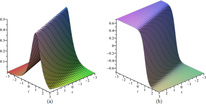
(a) 3D representation of solution (14) in the form of the bright soliton for a 1 = γ 1 = 1.5 , k = - 1 , ω = θ 0 = 1 , λ 1 = 2.5 , η = 3 . (b) 3D representation of solution (20) in form of dark soliton for a 1 = = 0.5 , k = - 1 , γ 1 = θ 0 = ω = 1 , λ 1 = - 2 , η = 3 ..

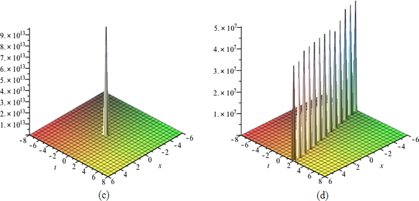
(c) 3D representation of solution (26) in the form of singular soliton as a 1 = γ 1 = 1.5 , k = ω = θ 0 = 1 , λ 1 = 2.5 , η = 3 . (d) 3D representation of solution (31) in the form of singular soliton for a 1 = 0.5 , k = - 1 , γ 1 = θ 0 = ω = 1 , λ 1 = - 2 , η = 3 .

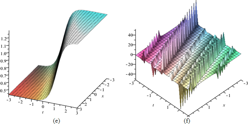
(e) 3D portrayal of combo optical soliton solution (45). (f) 3D representation of periodic singular solution (57).

Fig. 3(e) represents combo soliton solution (45) for $a_{1} = γ_{1} = 1.5, k = θ_{0} = ω = 1, λ_{1} = 2.5, d = 1.7, η = 3$ .

2.6

2.6 Modified Mapping Technique

Assuming PDE be of the following form

(47)

G (g, h, g_{t}, h_{t}, g_{x}, h_{x}, g_{xxx}, h_{xxx}, . . .) = 0 .

Let the solution of $(47)$ is written as
(48)
$\begin{matrix} g (x, t) = g (ϑ) = \sum_{i = 0}^{n_{1}} C_{i} P^{i} (ϑ), \\ h (x, t) = h (ϑ) = \sum_{i = 0}^{n_{2}} D_{i} P^{i} (ϑ), \end{matrix}$ where $ϑ = x - η t, C_{i}, D_{i}$ and $η$ are arbitrary constants. Let the first derivative of P be
(49)
$P'^{2} = {aP}^{2} + \frac{1}{2} {bP}^{4} + c,$ with constants $a, b$ , and c.
Utilizing Eq. $(48)$ in Eq. $(47)$ , by which Eq. $(47)$ changes into an ODE and $n_{1}$ and $n_{2}$ can be calculated by balancing principle.

Thus, the solution of (8) is considered as

(50)

Q_{i} (ϑ) = C_{0} + C_{1} P (ϑ) + D_{1} P^{- 1} (ϑ),

where

C_{0}, C_{1}

and

D_{1}

are constants.

Eq. (8) can be rewritten as

(51)

{AQ}_{i}^{''} + {BQ}_{i} + {CQ}_{i}^{3} = 0,

where

(52)

A = a_{1}, B = - (a_{i} k^{2} - ω), C = - k (λ_{i} + γ_{i}) .

Putting (50) into (51) and utilizing $(49)$ , we have $\begin{matrix} 2 {cAD}_{1} + {CD}_{1}^{3} = 0, \\ 3 {CC}_{0} D_{1}^{2} = 0, \\ {aAD}_{1} + 3 {CC}_{0}^{2} + 3 {CC}_{1} D_{1}^{2} + {BD}_{1} = 0, \\ {BC}_{0} + {CC}_{0}^{3} + 6 {CC}_{0} C_{1} D_{1} = 0, \\ {aAC}_{1} + {BC}_{1} + 3 {CC}_{0}^{2} C_{1} + 3 {CC}_{1}^{2} D_{1} = 0, \\ 3 {CC}_{0} C_{1}^{2} = 0, \\ {bAC}_{1} + {CC}_{1}^{3} = 0 . \end{matrix}$

From these equations, we get

(53)

C_{0} = 0, C_{1} = \sqrt{\frac{{ba}_{1}}{k (λ_{i} + γ_{i})}}, D_{1} = \sqrt{\frac{2 {ca}_{1}}{k (λ_{i} + γ_{i})}},

with constraint condition

(54)

aA + 3 {CC}_{1} D_{1} + B = 0 .

Case-1: $P (ϑ) = sn (ϑ)$ or $P (ϑ) = cd (ϑ)$ , we have $a = - (1 + r^{2}), b = 2 r^{2}$ and $c = 1$ . Now solutions of the $(2)$ are

(55)

ϕ (x, t) = \sqrt{\frac{2 a_{1}}{k (λ_{1} + γ_{1})}} [rsn (x - η t) + ns (x - η t)] e^{ι (- kx + ω t + θ_{0})},

and

(56)

ψ (x, t) = \sqrt{\frac{2 a_{2}}{k (λ_{2} + γ_{2})}} [rsn (x - η t) + ns (x - η t)] e^{ι (- kx + ω t + θ_{0})} .

When $r \to 0$ , then $ns \to \csc, (55)$ and $(56)$ yield the following singular solutions

(57)

ϕ (x, t) = \sqrt{\frac{2 a_{1}}{k (λ_{1} + γ_{1})}} \csc (x - η t) e^{ι (- kx + ω t + θ_{0})},

and

(58)

ψ (x, t) = \sqrt{\frac{2 a_{2}}{k (λ_{2} + γ_{2})}} \csc (x - η t) e^{ι (- kx + ω t + θ_{0})} .

When $r \to 1$ then $sn \to \tanh$ and $ns \to \coth, (55)$ and $(56)$ present dark-singular combo solitons as

(59)

ϕ (x, t) = \sqrt{\frac{2 a_{1}}{k (λ_{1} + γ_{1})}} [\tanh (x - η t) + \coth (x - η t)] e^{ι (- kx + ω t + θ_{0})},

and

(60)

ψ (x, t) = \sqrt{\frac{2 a_{2}}{k (λ_{2} + γ_{2})}} [\tanh (x - η t) + \coth (x - η t)] e^{ι (- kx + ω t + θ_{0})} .

(61)

ϕ (x, t) = \sqrt{\frac{2 a_{1}}{k (λ_{1} + γ_{1})}} [rcd (x - η t) + dc (x - η t)] e^{ι (- kx + ω t + θ_{0})},

and

(62)

ψ (x, t) = \sqrt{\frac{2 a_{2}}{k (λ_{2} + γ_{2})}} [rcd (x - η t) + dc (x - η t)] e^{ι (- kx + ω t + θ_{0})} .

When $r \to 0, dc \to \sec$ , which gives the following periodic singular solutions

(63)

ϕ (x, t) = \sqrt{\frac{2 a_{1}}{k (λ_{1} + γ_{1})}} \sec (x - η t) e^{ι (- kx + ω t + θ_{0})},

and

(64)

ψ (x, t) = \sqrt{\frac{2 a_{2}}{k (λ_{2} + γ_{2})}} \sec (x - η t) e^{ι (- kx + ω t + θ_{0})} .

When $r \to 1$ , the following solution are obtained

(65)

ϕ (x, t) = \sqrt{\frac{2 a_{1}}{k (λ_{1} + γ_{1})}} 2 e^{ι (- kx + ω t + θ_{0})},

and

(66)

ψ (x, t) = \sqrt{\frac{2 a_{2}}{k (λ_{2} + γ_{2})}} 2 e^{ι (- kx + ω t + θ_{0})} .

Fig. 3(f) represents the periodic singular solution (57) while Figs. 4(g) and 4(h) represent dark-singular soliton (59) and periodic singular solution (63) respectively, with $a_{1} = γ_{1} = 1.5, k = θ_{0} = ω = 1, λ_{1} = 2.5, η = 3$ .

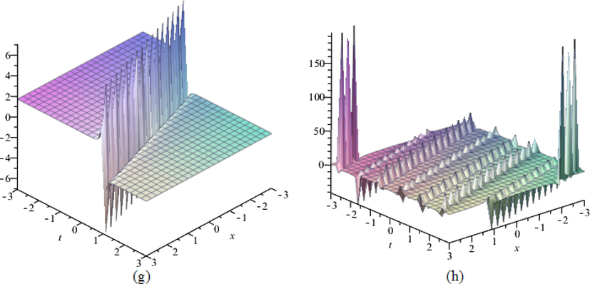
(g) 3D portrayal of dark-singular soliton solution (59). (h) 3D representation of periodic singular solution (63).

Case-2: When $P (ϑ) = cn (ϑ)$ , then $a = 2 r^{2} - 1, b = - 2 r^{2}$ and $c = 1 - r^{2}$ . So

(67)

ϕ (x, t) = \sqrt{- \frac{2 a_{1}}{k (λ_{1} + γ_{1})}} [rcn (x - η t) + \sqrt{r^{2} - 1} nc (x - η t)] e^{ι (- kx + ω t + θ_{0})},

and

(68)

ψ (x, t) = \sqrt{- \frac{2 a_{2}}{k (λ_{2} + γ_{2})}} [rcn (x - η t) + \sqrt{r^{2} - 1} nc (x - η t)] e^{ι (- kx + ω t + θ_{0})} .

When $r \to 0$ , we obtain the same periodic singular solution as $(57)$ and $(58)$ .

When $r \to 1$ , the bright soliton solutions are retrieved as

(69)

ϕ (x, t) = \sqrt{- \frac{2 a_{1}}{k (λ_{1} + γ_{1})}} sech (x - η t) e^{ι (- kx + ω t + θ_{0})},

and

(70)

ψ (x, t) = \sqrt{- \frac{2 a_{2}}{k (λ_{2} + γ_{2})}} sech (x - η t) e^{ι (- kx + ω t + θ_{0})} .

Fig. 5(i) portrays the bright soliton solution (69) with $a_{1} = γ_{1} = 1.5, k = - 1, θ_{0} = ω = 1, λ_{1} = 2.5, η = 3$ .

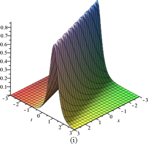
(i) 3D portrayal of bright soliton solution (69).

Case-3: When $P (ϑ) = cs (ϑ)$ , then $a = 2 - r^{2}, b = 2$ and $c = 1 - r^{2}$ . So

(71)

ϕ (x, t) = \sqrt{- \frac{2 a_{1}}{k (λ_{1} + γ_{1})}} [rcs (x - η t) + \sqrt{1 - r^{2}} sc (x - η t)] e^{ι (- kx + ω t + θ_{0})},

and

(72)

ψ (x, t) = \sqrt{- \frac{2 a_{2}}{k (λ_{2} + γ_{2})}} [rcs (x - η t) + \sqrt{1 - r^{2}} sc (x - η t)] e^{ι (- kx + ω t + θ_{0})} .

Substituting $r \to 0$ in $(71)$ and $(72)$ yield the following periodic singular solutions

(73)

ϕ (x, t) = \sqrt{\frac{2 a_{1}}{k (λ_{1} + γ_{1})}} [\cot (x - η t)] e^{ι (- kx + ω t + θ_{0})},

and

(74)

ψ (x, t) = \sqrt{\frac{2 a_{2}}{k (λ_{2} + γ_{2})}} [\cot (x - η t)] e^{ι (- kx + ω t + θ_{0})} .

Substituting $r \to 1$ in $(71)$ and $(72)$ yield the following singular soliton solutions

(75)

ϕ (x, t) = \sqrt{\frac{2 a_{1}}{k (λ_{1} + γ_{1})}} csch (x - η t) e^{ι (- kx + ω t + θ_{0})},

and

(76)

ψ (x, t) = \sqrt{\frac{2 a_{2}}{k (λ_{2} + γ_{2})}} csch (x - η t) e^{ι (- kx + ω t + θ_{0})} .

Figs. 6(j) represents the periodic singular solution (73) for $a_{1} = γ_{1} = 1.5, k = θ_{0} = ω = 1, λ_{1} = 2.5, η = 3$ .

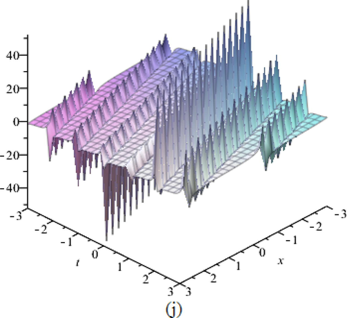
(j) 3D representation of periodic singular solution (73).

3 Conclusion

This study takes up the KNE without FWM in birefringent fibers. Three proposed methods are fruitfully applied to recover optical soliton solutions for the present model. Comparing the obtained results with those in earlier study, it is demonstrated that our results are new and not studied earlier. From these integration schemes dark, bright, singular, bright-singular and periodic singular combo soliton solutions are retrieved. These techniques are concise, efficient and the solutions opens up wide opportunities for further studies.

Declaration of Competing Interest

The authors declare that they have no known competing financial interests or personal relationships that could have appeared to influence the work reported in this paper.

References

Abbagari S., Houwe A., Rezazadeh H., Bekir A., Bouetou T.B., Crépin K.T., . Optical soliton to multi-core (coupling with all the neighbors) directional couplers and modulation instability. European Phys. J. Plus. 2021;136(3):1-19.
[Google Scholar]
Ahmed H.M., Rabie W.B., Arnous A.H., Wazwaz A.M., . Optical solitons in birefringent fibers of Kaup-Newell’s equation with extended simplest equation method. Physica Scr.. 2020;95:115214
[Google Scholar]
An T., Shahen N.H.M., Ananna S.N., Hossain M.F., Muazu T., . Exact and explicit travelling-wave solutions to the family of new 3D fractional WBBM equations in mathematical physics. Results Phys.. 2020;19:103517
[Google Scholar]
Arshad M., Seadawy A.R., Lu D., . Elliptic function and solitary wave solutions of the higher-order nonlinear Schrödinger dynamical equation with fourth-order dispersion and cubic-quintic nonlinearity and its stability. European Phys. J. Plus. 2017;132(8):1-11.
[Google Scholar]
Arshed S., Biswas A., Abdelaty M., Zhou Q., Moshokoa S.P., Belic M., . Sub-pico second chirp-free optical solitons with Kaup-Newell equation using a couple of strategic algorithms. Optik.. 2018;172:766-771.
[Google Scholar]
Awan A.U., Tahir M., Rehman H.U., . Singular and bright-singular combo optical solitons in birefringent fibers to the Biswas-Arshed equation. Optik.. 2020;210:164489
[Google Scholar]
Awan A.U., Tahir M., Abro K.A., . Multiple soliton solutions with chiral nonlinear Schrodinger’s equation in (2+1)-dimensions. European J. Mech. - B/Fluids. 2021;85:68-75.
[Google Scholar]
Bhrawy A.H., Alshaery A.A., Hilal E.M., Savescu M., Milovic D., Khan K.R., Mahmood M.F., Jovanoski Z., Biswas A., . Optical solitons in birefringent fibers with spatio-temporal disperesion. Optik.. 2014;125(17):4935-4944.
[Google Scholar]
Biswas A., Ekici M., Sonmezoglu A., Alqahtani R.T., . Sub-pico second chirped optical solitons in monomode fibers with Kaup-Newell equation by extended trial function method. Optik.. 2018;168:208-216.
[Google Scholar]
Biswas A., Yildirim Y., Yasar E., Zhou Q., Moshokoa S.P., Belic M., . Sub pico-second pulses in mono-mode optical fibers with Kaup-Newell equation by a couple of integration schemes. Optik.. 2018;167:121-128.
[Google Scholar]
Delgado V.F.M., Aguilar J.F.G., Hernandez M.A.T., Baleanu D., . Modeling the fractional non-linear Schrodinger equation via Liouville-Caputo fractional derivative. Optik.. 2018;162:1-7.
[Google Scholar]
Ghanbari B., Aguilar J.F.G., . Optical soliton solutions for the nonlinear Radhakrishnan-Kundu-Lakshmanan equation. Modern Phys. Letters B. 2019;33(32):1950402.
[Google Scholar]
Hosseini K., Aligoli M., Mirzazadeh M., Eslami M., Gomez-Aguilar J.F., . Dynamics of rational solutions in a new generalized Kadomtsev-Petviashvili equation. Mod. Phys. Lett. B. 2019;33(35):1950437.
[Google Scholar]
Hosseini K., Salahshour S., Mirzazadeh M., Ahmadian A., Baleanu D., Khoshrang A., . The (2+ 1)-dimensional Heisenberg ferromagnetic spin chain equation: its solitons and Jacobi elliptic function solutions. European Phys. J. Plus. 2021;136(2):1-9.
[Google Scholar]
Hussain T., Awan A.U., Abro K.A., Ozair M., Manzoor M., . A mathematical and parametric study of epidemiological smoking model: a deterministic stability and optimality for solutions. European Phys. J. Plus. 2021;136:11.
[Google Scholar]
Jawad A.J.M., Al Azzawi F.J.I., Biswas A., Khan S., Zhou Q., Moshokoa S.P., Belic M.R., . Bright and singular optical solitons for Kaup-Newell equation with two fundamental integration norms. Optik.. 2019;182:594-597.
[Google Scholar]
Liu J.G., Zhu W.H., Osman M.S., Ma W.X., . An explicit plethora of different classes of interactive lump solutions for an extension form of 3D-Jimbo-Miwa model. European Phys. J. Plus. 2020;135(5):1-9.
[Google Scholar]
Martinez H.Y., Aguilar J.F.G., Baleanu D., . Beta-derivative and sub-equation method applied to the optical solitons in medium with parabolic law nonlinearity and higher order dispersion. Optik.. 2018;155:357-365.
[Google Scholar]
Memon I.Q., Abro K.A., Solangi M.A., Shaikh A.A., . Functional shape effects of nanoparticles on nanofluid suspended in ethylene glycol through Mittage-Leffler approach. Phys. Scr.. 2020;96(2):025005
[Google Scholar]
Morales-Delgado V.F., Gomez-Aguilar J.F., Baleanu D., . A new approach to exact optical soliton solutions for the nonlinear Schrodinger equation. Eur. Phys. J. Plus. 2018;133(5):189.
[Google Scholar]
Rehman H.U., Jafar S., Javed A., Hussain S., Tahir M., . New optical solitons of Biswas-Arshed equation using different techniques. Optik.. 2019;206:163670
[Google Scholar]
Rehman H.U., Saleem M.S., Zubair M., Jafar S., Latif I., . Optical solitons with Biswas-Arshed model using mapping method. Optik.. 2019;194:163091
[Google Scholar]
Rehman H.U., Ullah N., Asjad M.I., . Highly dispersive optical solitons using Kudryashov’s method. Optik.. 2019;199:163349
[Google Scholar]
Rehman H.U., Tahir M., Bibi M., Ishfaq Z., . Optical solitons to the Biswas-Arshed model in birefringent fibers using couple of integration techniques. Optik.. 2020;218:164894
[Google Scholar]
Rehman H.U., Ullah N., Asjad M.I., . Optical solitons of Biswas-Arshed equation in birefringent fibers using extended direct algebraic method. Optik.. 2020;226:165378
[Google Scholar]
Rehman H.U., Ullah N., Asjad M.I., Akgul A., . Exact solutions of convective-diffusive Cahn-Hilliard equation using extended direct algebraic method. Numerical Methods Partial Differential Equations. 2020;1–16
[CrossRef] [Google Scholar]
Rehman H.U., Younis M., Jafar S., Tahir M., Saleem M.S., . Optical solitons of Biswas-Arshed model in birefringent fibers without four-wave mixing. Optik.. 2020;213:164669
[Google Scholar]
Sedeeg A.K.H., Nuruddeen R.I., Aguilar J.F.G., . Generalized optical soliton solutions to the (3+1)-dimensional resonant nonlinear Schrodinger equation with Kerr and parabolic law nonlinearities. Optical Quantum Electron.. 2019;51(6):173.
[Google Scholar]
Shahen N.H.M., Bashar M.H., Ali M.S., . Dynamical analysis of long-wave phenomena for the nonlinear conformable space-time fractional (2+1)-dimensional AKNS equation in water wave mechanics. Heliyon. 2020;6(10):e05276
[Google Scholar]
Syed T.S., Abro K.A., Sikandar A., . Role of single slip assumption on the viscoelastic liquid subject to non-integer differentiable operators. Math. Meth. Appl. Sci.. 2021;1–16:7164.
[Google Scholar]
Tahir M., Awan A.U., . Analytical solitons with the Biswas-Milovic equation in the presence of spatio-temporal dispersion in non-Kerr law media. Eur. Phys. J. Plus. 2019;134:464.
[Google Scholar]
Tahir M., Awan A.U., . Optical travelling wave solutions for the Biswas-Arshed model in Kerr and non Kerr-law media. Pramana.. 2020;94(1):29.
[Google Scholar]
Tahir M., Awan A.U., . Optical dark and singular solitons to the Biswas-Arshed equation in birefringent fibers without four-wave mixing. Optik.. 2020;207:164421
[Google Scholar]
Tahir M., Awan A.U., Rehman H.U., . Optical solitons to Kundu-Eckhaus equation in birefringent fibers without four-wave mixing. Optik.. 2019;199:163297
[Google Scholar]
Tahir M., Awan A.U., Rehman H.U., . Dark and singular optical solitons to the Biswas-Arshed model with Kerr and power law nonlinearity. Optik.. 2019;185:777-783.
[Google Scholar]
Triki H., Biswas A., Zhou Q., Moshokoa S.P., Belic M., . Chirped envelope optical solitons for Kaup-Newell equation. Optik.. 2019;177:1-7.
[Google Scholar]
Yepez-Martinez H., Gomez-Aguilar J.F., Atangana A., . First integral method for non-linear differential equations with conformable derivative. Math. Modelling Natural Phenomena. 2018;13(1):14.
[Google Scholar]
Yildirim Y., Biswas A., Zhouf Q., Alshomrani A.S., Belic M.R., . Sub pico-second optical pulses in birefringent fibers for Kaup-Newell equation with cutting-edge integration technologies. Results Phys.. 2019;15:102660
[Google Scholar]
Yoku A., Durur H., Abro K.A., Kaya D., . Role of Gilson-Pickering equation for the different types of soliton solutions: A nonlinear analysis. Eur. Phys. J. Plus. 2020;135(8):1-19.
[Google Scholar]

Introduction

Mathematical Analysis

Bright Soliton
Dark Soliton
Singular Soliton (Type-I)
Singular Soliton (Type-II)
Kudryashov’s Method
Modified Mapping Technique

Conclusion

Fulltext Views
5

PDF downloads
4

View/Download PDF
Download Citations

BibTeX
RIS

Show Sections

[1] Abbagari S., Houwe A., Rezazadeh H., Bekir A., Bouetou T.B., Crépin K.T., . Optical soliton to multi-core (coupling with all the neighbors) directional couplers and modulation instability. European Phys. J. Plus. 2021;136(3):1-19.
[Google Scholar]

[2] Ahmed H.M., Rabie W.B., Arnous A.H., Wazwaz A.M., . Optical solitons in birefringent fibers of Kaup-Newell’s equation with extended simplest equation method. Physica Scr.. 2020;95:115214
[Google Scholar]

[3] An T., Shahen N.H.M., Ananna S.N., Hossain M.F., Muazu T., . Exact and explicit travelling-wave solutions to the family of new 3D fractional WBBM equations in mathematical physics. Results Phys.. 2020;19:103517
[Google Scholar]

[4] Arshad M., Seadawy A.R., Lu D., . Elliptic function and solitary wave solutions of the higher-order nonlinear Schrödinger dynamical equation with fourth-order dispersion and cubic-quintic nonlinearity and its stability. European Phys. J. Plus. 2017;132(8):1-11.
[Google Scholar]

[5] Arshed S., Biswas A., Abdelaty M., Zhou Q., Moshokoa S.P., Belic M., . Sub-pico second chirp-free optical solitons with Kaup-Newell equation using a couple of strategic algorithms. Optik.. 2018;172:766-771.
[Google Scholar]

[6] Awan A.U., Tahir M., Rehman H.U., . Singular and bright-singular combo optical solitons in birefringent fibers to the Biswas-Arshed equation. Optik.. 2020;210:164489
[Google Scholar]

[7] Awan A.U., Tahir M., Abro K.A., . Multiple soliton solutions with chiral nonlinear Schrodinger’s equation in (2+1)-dimensions. European J. Mech. - B/Fluids. 2021;85:68-75.
[Google Scholar]

[8] Bhrawy A.H., Alshaery A.A., Hilal E.M., Savescu M., Milovic D., Khan K.R., Mahmood M.F., Jovanoski Z., Biswas A., . Optical solitons in birefringent fibers with spatio-temporal disperesion. Optik.. 2014;125(17):4935-4944.
[Google Scholar]

[9] Biswas A., Ekici M., Sonmezoglu A., Alqahtani R.T., . Sub-pico second chirped optical solitons in monomode fibers with Kaup-Newell equation by extended trial function method. Optik.. 2018;168:208-216.
[Google Scholar]

[10] Biswas A., Yildirim Y., Yasar E., Zhou Q., Moshokoa S.P., Belic M., . Sub pico-second pulses in mono-mode optical fibers with Kaup-Newell equation by a couple of integration schemes. Optik.. 2018;167:121-128.
[Google Scholar]

[11] Delgado V.F.M., Aguilar J.F.G., Hernandez M.A.T., Baleanu D., . Modeling the fractional non-linear Schrodinger equation via Liouville-Caputo fractional derivative. Optik.. 2018;162:1-7.
[Google Scholar]

[12] Ghanbari B., Aguilar J.F.G., . Optical soliton solutions for the nonlinear Radhakrishnan-Kundu-Lakshmanan equation. Modern Phys. Letters B. 2019;33(32):1950402.
[Google Scholar]

[13] Hosseini K., Aligoli M., Mirzazadeh M., Eslami M., Gomez-Aguilar J.F., . Dynamics of rational solutions in a new generalized Kadomtsev-Petviashvili equation. Mod. Phys. Lett. B. 2019;33(35):1950437.
[Google Scholar]

[14] Hosseini K., Salahshour S., Mirzazadeh M., Ahmadian A., Baleanu D., Khoshrang A., . The (2+ 1)-dimensional Heisenberg ferromagnetic spin chain equation: its solitons and Jacobi elliptic function solutions. European Phys. J. Plus. 2021;136(2):1-9.
[Google Scholar]

[15] Hussain T., Awan A.U., Abro K.A., Ozair M., Manzoor M., . A mathematical and parametric study of epidemiological smoking model: a deterministic stability and optimality for solutions. European Phys. J. Plus. 2021;136:11.
[Google Scholar]

[16] Jawad A.J.M., Al Azzawi F.J.I., Biswas A., Khan S., Zhou Q., Moshokoa S.P., Belic M.R., . Bright and singular optical solitons for Kaup-Newell equation with two fundamental integration norms. Optik.. 2019;182:594-597.
[Google Scholar]

[17] Liu J.G., Zhu W.H., Osman M.S., Ma W.X., . An explicit plethora of different classes of interactive lump solutions for an extension form of 3D-Jimbo-Miwa model. European Phys. J. Plus. 2020;135(5):1-9.
[Google Scholar]

[18] Martinez H.Y., Aguilar J.F.G., Baleanu D., . Beta-derivative and sub-equation method applied to the optical solitons in medium with parabolic law nonlinearity and higher order dispersion. Optik.. 2018;155:357-365.
[Google Scholar]

[19] Memon I.Q., Abro K.A., Solangi M.A., Shaikh A.A., . Functional shape effects of nanoparticles on nanofluid suspended in ethylene glycol through Mittage-Leffler approach. Phys. Scr.. 2020;96(2):025005
[Google Scholar]

[20] Morales-Delgado V.F., Gomez-Aguilar J.F., Baleanu D., . A new approach to exact optical soliton solutions for the nonlinear Schrodinger equation. Eur. Phys. J. Plus. 2018;133(5):189.
[Google Scholar]

[21] Rehman H.U., Jafar S., Javed A., Hussain S., Tahir M., . New optical solitons of Biswas-Arshed equation using different techniques. Optik.. 2019;206:163670
[Google Scholar]

[22] Rehman H.U., Saleem M.S., Zubair M., Jafar S., Latif I., . Optical solitons with Biswas-Arshed model using mapping method. Optik.. 2019;194:163091
[Google Scholar]

[23] Rehman H.U., Ullah N., Asjad M.I., . Highly dispersive optical solitons using Kudryashov’s method. Optik.. 2019;199:163349
[Google Scholar]

[24] Rehman H.U., Tahir M., Bibi M., Ishfaq Z., . Optical solitons to the Biswas-Arshed model in birefringent fibers using couple of integration techniques. Optik.. 2020;218:164894
[Google Scholar]

[25] Rehman H.U., Ullah N., Asjad M.I., . Optical solitons of Biswas-Arshed equation in birefringent fibers using extended direct algebraic method. Optik.. 2020;226:165378
[Google Scholar]

[26] Rehman H.U., Ullah N., Asjad M.I., Akgul A., . Exact solutions of convective-diffusive Cahn-Hilliard equation using extended direct algebraic method. Numerical Methods Partial Differential Equations. 2020;1–16
[CrossRef] [Google Scholar]

[27] Rehman H.U., Younis M., Jafar S., Tahir M., Saleem M.S., . Optical solitons of Biswas-Arshed model in birefringent fibers without four-wave mixing. Optik.. 2020;213:164669
[Google Scholar]

[28] Sedeeg A.K.H., Nuruddeen R.I., Aguilar J.F.G., . Generalized optical soliton solutions to the (3+1)-dimensional resonant nonlinear Schrodinger equation with Kerr and parabolic law nonlinearities. Optical Quantum Electron.. 2019;51(6):173.
[Google Scholar]

[29] Shahen N.H.M., Bashar M.H., Ali M.S., . Dynamical analysis of long-wave phenomena for the nonlinear conformable space-time fractional (2+1)-dimensional AKNS equation in water wave mechanics. Heliyon. 2020;6(10):e05276
[Google Scholar]

[30] Syed T.S., Abro K.A., Sikandar A., . Role of single slip assumption on the viscoelastic liquid subject to non-integer differentiable operators. Math. Meth. Appl. Sci.. 2021;1–16:7164.
[Google Scholar]

[31] Tahir M., Awan A.U., . Analytical solitons with the Biswas-Milovic equation in the presence of spatio-temporal dispersion in non-Kerr law media. Eur. Phys. J. Plus. 2019;134:464.
[Google Scholar]

[32] Tahir M., Awan A.U., . Optical travelling wave solutions for the Biswas-Arshed model in Kerr and non Kerr-law media. Pramana.. 2020;94(1):29.
[Google Scholar]

[33] Tahir M., Awan A.U., . Optical dark and singular solitons to the Biswas-Arshed equation in birefringent fibers without four-wave mixing. Optik.. 2020;207:164421
[Google Scholar]

[34] Tahir M., Awan A.U., Rehman H.U., . Optical solitons to Kundu-Eckhaus equation in birefringent fibers without four-wave mixing. Optik.. 2019;199:163297
[Google Scholar]

[35] Tahir M., Awan A.U., Rehman H.U., . Dark and singular optical solitons to the Biswas-Arshed model with Kerr and power law nonlinearity. Optik.. 2019;185:777-783.
[Google Scholar]

[36] Triki H., Biswas A., Zhou Q., Moshokoa S.P., Belic M., . Chirped envelope optical solitons for Kaup-Newell equation. Optik.. 2019;177:1-7.
[Google Scholar]

[37] Yepez-Martinez H., Gomez-Aguilar J.F., Atangana A., . First integral method for non-linear differential equations with conformable derivative. Math. Modelling Natural Phenomena. 2018;13(1):14.
[Google Scholar]

[38] Yildirim Y., Biswas A., Zhouf Q., Alshomrani A.S., Belic M.R., . Sub pico-second optical pulses in birefringent fibers for Kaup-Newell equation with cutting-edge integration technologies. Results Phys.. 2019;15:102660
[Google Scholar]

[39] Yoku A., Durur H., Abro K.A., Kaya D., . Role of Gilson-Pickering equation for the different types of soliton solutions: A nonlinear analysis. Eur. Phys. J. Plus. 2020;135(8):1-19.
[Google Scholar]

A non-linear study of optical solitons for Kaup-Newell equation without four-wave mixing

Abstract

Keywords

Nonlinear

Birefringent fibers

Optical solitons

Kaup-Newell Equation

Four-Wave Mixing

1 Introduction

2 Mathematical Analysis

2.1 Bright Soliton

2.2 Dark Soliton

2.3 Singular Soliton (Type-I)

2.4 Singular Soliton (Type-II)

2.5 Kudryashov’s Method

2.6 Modified Mapping Technique

3 Conclusion

Declaration of Competing Interest

References

Suggested read for related articles: