

Translate this page into:
A new third order convergent numerical solver for continuous dynamical systems
⁎Corresponding author. sania.qureshi@faculty.muet.edu.pk (Sania Qureshi),
-
Received: ,
Accepted: ,
This article was originally published by Elsevier and was migrated to Scientific Scholar after the change of Publisher.
Peer review under responsibility of King Saud University.
Abstract
A new numerical solver with third order convergence has been proposed. The solver is consistent, stable, and possesses smaller error bounds. Error analysis of the solver has been carried in detail. The performance of the solver is better than many existing solvers having similar characteristics.
Abstract
Continuous dynamical systems are attempted to solve via proposed third order convergent numerical solver. The solver is shown to possess third order convergence on the basis of containing term in the leading coefficient of the local truncation error which has further been employed for the local and global error bounds whereas its increment function is found to be Lipchitz continuous. Consistency of the solver has extensively been discussed using Taylor’s series expansion. The necessary and sufficient conditions for the solver to be stable have been proved accompanying the linear stability function obtained via Dahlquist test problem. In order to illustrate the performance of the solver, few scalar and vector-valued dynamical systems of both linear and nonlinear nature have numerically been solved in comparison to two well-known numerical solvers having same order of convergence as that of the proposed solver. Whereupon, the proposed solver is found to contain the smallest errors. The analysis of comparison is based upon three kinds of errors; namely, maximum absolute global relative error, absolute relative error determined at the final nodal point along the integration interval and the -error norm. MATLAB software having version 9.3.0.713579 (R2017b), using Intel(R) Core(TM) i3-4500U processor running on 1.70 GHz has been used.
Keywords
Differential equations
Local error
Global error
Lipchitz continuity
Stability

1 Introduction
Mathematical models containing ordinary differential equations (ODEs) play a vital role in various fields of study. Areas including engineering, applied mathematics, bio-medical, statistical mechanics, quantum mechanics, economics, image processing, control theory, and many others are not considered to be complete without inclusion of subjects on differential equations and their applications in respective fields (Amann, 2011; Butcher, 2016; Hirsch et al., 2012; Jordan and Peter, 1999; Mermoud and Lausanne, 2015; Shampine, 2018; Stickler and Ewald, 2014; Teschl, 2000). Unfortunately, large quantity of such physical and natural models have no closed form solutions due to one or other type of non-linearity associated with the models.
Due to the universal acceptance of the importance of such mathematical models, many researchers have devised new solvers to get the desired solutions of the models under their study whereas others have substantially improved the performance of many existing solvers with regard to the convergence order, computational complexity, stability, consistency and error bounds.
In order to solve the scalar and continuous dynamical systems, the authors in (Ma and Simos, 2017; Rabiei and Fudziah, 2012; Rabiei et al., 2012a; Rabiei et al., 2012b) have improved the efficiency for the well-known family of explicit linear Runge-Kutta numerical solvers by decreasing the number of slope evaluations in its each application while maintaining the convergence order whereas others in (Qureshi and Ramos, 2018; Ramos et al., 2010; Ramos and Jesús, 2008) have devised new nonlinear numerical solvers to deal with the autonomous and non-autonomous continuous dynamical systems having singular or singularly perturbed solutions at some point of the time interval . Rational block and trigonometrically fitted solvers have recently been proposed for the efficient solutions of initial value problems having oscillatory solutions, in particular (Ehigie et al., 2017; Jesús et al., 2017; Jesús et al., 2008; Kalogiratou, 2016; Tsitouras and Simos, 2018). Apart from this, the most recent work is discussed in (Bakodah, 2018; Liu, 2018; Moutsinga et al., 2018; Neštický et al., 2017; Nuruddeen and Nass, 2017; Qureshi and Emmanuel, 2018; Qureshi et al., 2018; Raza and Khan, 2019).
There are many reasons for one numerical solver to become superior over the other. One of the major reasons is the convergence order (a numerical solver is of order r if the error is proved to have as for a constant time step length ) which shows the rate at which the numerical error in an application of a constant time step length solver along decreases as a consequence of decreasing the time step length h. It is therefore a numerical solver having first order convergence would experience halving of the numerical error when the time step length h is halved. Likewise, second order convergent numerical solver would yield the error being multiplied by a factor of when h is halved.
Nevertheless, the numerical errors observed in practice could be different (worse or better) from those predicted and it is because the convergence orders are asymptotic results and apply only when . There is always an asymptotic error constant that depends on the solver and the equation which decides the size of the true error. This is the reason for two numerical solvers of same convergence order to have entirely different behavior in errors when they are used for solving the same initial value problem.
The present study aims to propose a new numerical solver having third order convergence. The proposed solver is of explicit linear single-step structure but the inclusion of partial derivative with respect to the second variable of the slope u makes it well comparable with existing third order convergent solvers of similar characteristics. Thus, it can be included in the family of explicit single-step numerical solvers which are considered to be cost effective and easy to be implemented within a computer code.
2 Derivation of the proposed numerical solver
Suppose that a well-defined initial value problem is given as
Further, it is assumed that the problem (1) possesses a unique continuously differentiable solution where for is taken to be the approximation to the analytical (exact) solution at over the associated interval of integration with as a fixed time step length used at each step of the integration.
A numerical solver having explicit nature for single-step structure is generally formulated as:
3 Analysis for the proposed solver
For the required analysis, some definitions and the related theorems have been stated.
3.1 Consistency
A numerical solver used for finding the solution of an initial value problem in ODEs is said to be consistent if
The increment function of the proposed solver is as follows:
3.2 Stability
Suppose that
be real numbers satisfying
Using the assumption presented in the above Theorem 1, we can write the following:
Suppose that
and
be two numerical solutions to the ODE
produced by a numerical solver with prescribed initial conditions
and
respectively such that
. The following condition
Using the above Theorem 2, the proposed solver would give us the following:
Further, the Dahlquist (Dahlquist, 1956) test problem
gives the following stability function for the proposed solver.
3.3 Error analysis
Suppose that and be any two points in the region S defined by , and that u is a Lipschitz continuous function on S such that , then the increment function is Lipschitz continuous, and where L and are, respectively, the Lipschitz constants for u and .
Employing the assumptions above, we get the following
This completes the proof for the increment function for the proposed solver to be Lipchitz continuous.
3.3.1 Error bounds
.
Suppose that
be the analytical (exact) solution of the underlying initial value problem at
and
be its corresponding numerical (approximate) solution obtained via a numerical solver. The global error
at
is defined as:
The local error
at
for a numerical solver like the one being studied in the present study is defined as:
The local error
of a numerical solver with order of accuracy r is also defined as
In order to obtain the local truncation error of the proposed integrator, a usual functional associated to the integrator has been considered, that is given below:
3.4 Convergence
The convergence for a numerical solver is guaranteed if for every initial value problem
with u being a Lipchitz continuous function, one obtains
Let us consider the proposed solver to be
Employing the Theorems 1 and 3, we obtain
Thus, the convergence of the proposed solver is verified for
4 Numerical experiments
Example 1. As shown in the Table 1 where the proposed solver shows the three-order decreasing behavior in the maximum absolute global relative errors
and in the errors computed at final nodal point
over
for every one-order decrease in the time step length h. The
-error norm
is shown in the last row. In addition, the computed errors are smallest in every case upon comparison with Heun and RK3HM (Wazwaz, 1990).
h
Heun
1.3048e−04 1.3048e−04 4.2260e−04
1.2425e−07 1.2425e−07 1.2441e−06
1.2352e−10 1.2352e−10 3.9015e−09
1.5984e−13 1.5970e−13 1.5036e−11
RK3HM
6.6502e−04 6.6502e−04 2.2030e−03
5.9464e−06 5.9464e−06 6.0417e−05
5.9024e−08 5.9024e−08 1.8898e−06
5.8979e−10 5.8979e−10 5.9693e−08
Proposed
2.3861e−05 8.2608e−06 8.1340e−05
2.6075e−08 1.3196e−08 2.8703e−07
2.6284e−11 1.3664e−11 9.1636e−10
5.8001e−14 4.9848e−14 5.6582e−12
Example 2. The observation for the linear problem with exponentially increasing solution based upon the Table 2 is more or less same as was in the former example.
h
Heun
6.4697e−05 6.4697e−05 8.3000e−05
6.8998e−08 6.8998e−08 2.2883e−07
6.9400e−11 6.9400e−11 7.1171e−10
1.3111e−13 1.3110e−13 4.4807e−12
RK3HM
2.2335e−03 2.2335e−03 4.1400e−03
2.4716e−05 2.4716e−05 1.3587e−04
2.4971e−07 2.4971e−07 4.3116e−06
2.4998e−09 2.4998e−09 1.3639e−07
Proposed
2.0183e−05 2.0183e−05 2.8573e−05
1.8702e−08 1.8702e−08 7.7040e−08
1.8535e−11 1.8535e−11 2.3974e−10
7.3701e−14 7.3664e−14 2.6931e−12
Example 3. The third initial value problem is structured in the form of a well-known nonlinear first order Riccati ODE. The proposed solver as shown in the Table 3 provides smallest magnitude of errors when compared with Heun and RK3HM methods. With one-order decrease in the time step length h, there are three-order decrease in the maximum absolute global relative errors and in the absolute relative errors determined at the final nodal point over
.
h
Heun
5.4644e−05 5.4644e−05 7.9834e−05
5.1896e−08 5.1896e−08 2.0943e−07
5.1603e−11 5.1603e−11 6.4899e−10
5.9233e−14 5.9172e−14 2.1293e−12
RK3HM
3.1635e−04 3.1635e−04 3.5014e−04
3.5178e−06 3.5178e−06 9.1739e−06
3.5477e−08 3.5477e−08 2.8310e−07
3.5505e−10 3.5505e−10 8.9296e−09
Proposed
6.4731e−06 3.2754e−06 1.0836e−05
8.3861e−09 1.9656e−09 4.2872e−08
8.3674e−12 2.1622e−12 1.3480e−10
1.2274e−14 1.2155e−14 4.2406e−13
Example 4. Here, the errors are computed for each unknown function
and
of the system as shown in the Tables 4–6 where decreasing behavior is clearly seen for all the solvers with the proposed solver having the smallest errors almost for every time step length h.
h
Heun
9.3411e+01 2.0974e+01
8.1516e−01 3.9783e+00
1.8376e−03 4.0405e−02
1.9256e−04 6.1855e−05
RK3HM
2.5717e+07 4.1029e+07
1.5990e+01 9.2617e+01
1.3092e+00 2.4304e+01
1.3639e+00 4.2652e−01
Proposed
2.6958e+01 1.7027e+01
3.6696e−01 1.7810e+00
5.1390e−04 1.1450e−02
5.3860e−05 1.7773e−05
h
Heun
3.5681e+00 1.0769e+00
8.9169e−02 8.3767e−03
7.4569e−05 8.8139e−06
7.5540e−08 8.8355e−09
RK3HM
2.5571e+07 1.8402e+07
2.7526e+00 1.8522e−01
4.8144e−02 1.6401e−03
4.9232e−04 2.1372e−05
Proposed
1.3021e+00 1.0083e+00
4.5361e−02 9.2884e−03
2.8136e−05 9.5089e−06
2.8907e−08 9.5067e−09
h
Heun
NaN 2.9205e+01
NaN 4.1695e+00
NaN 4.3136e−02
NaN 9.9840e−05
RK3HM
NaN 4.9949e+07
NaN 9.6513e+01
NaN 2.6034e+01
NaN 6.9477e−01
Proposed
NaN 2.1094e+01
NaN 1.8718e+00
NaN 1.2236e−02
NaN 2.7782e−05
Example 5. The angular displacement
for an undamped pendulum with a driving force
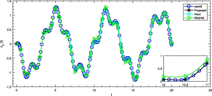
can be modeled in terms of a second order ODE as shown below. (See Fig 1)
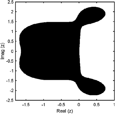
Stability region (shaded) for the proposed solver with
.
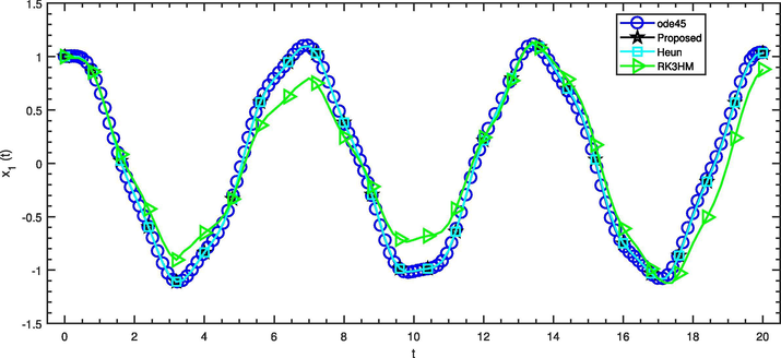
Comparison of solvers with
for the angular displacement
in the Example – 5.
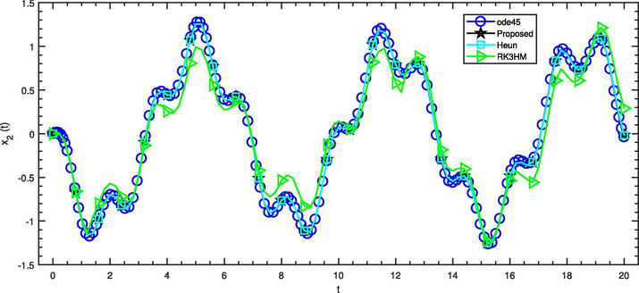
Comparison of solvers with
for the angular velocity
in the Example – 5.
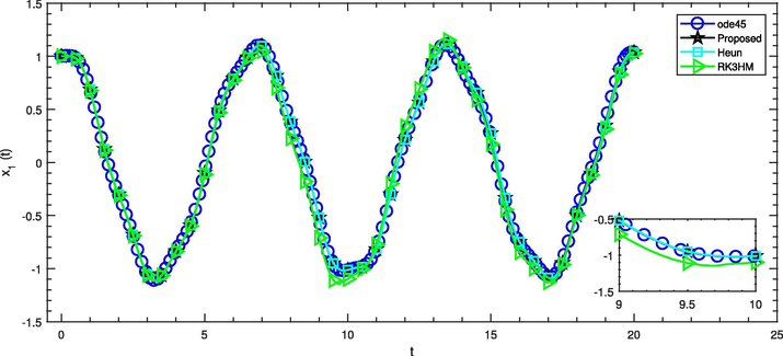
Comparison of solvers with
for the angular displacement
in the Example – 5.
Comparison of solvers with
for the angular velocity
in the Example – 5.
5 Conclusion
A numerical solver (6) having third order convergence has been proposed in the present study. Its error analysis led us to compute both local and global error bounds wherein the leading term in the local truncation error ensures the third order convergence of the solver. The increment function of the solver is shown to be Lipchitz continuous and the linear stability analysis has been carried out to get the stability region of the solver satisfying the condition .
Upon comparison with two well-known solvers (Heun and RK3HM) having similar characteristics as that of the proposed solver, it has been observed that the latter yielded smallest errors in both scalar and continuous dynamical systems of first and higher order as shown in the Tables 1–6. Thus, the proposed solver can be considered a member for the family of explicit linear single-step numerical solvers used to solve various continuous dynamical systems in the scientific fields.
Conflict of Interest
The authors declare no conflict of interest. Both authors have read and approved the final version of the present research work.
Acknowledgement
Sania Qureshi is grateful to Mehran University of Engineering and Technology, Jamshoro, Pakistan for the kind support and facilities provided to carry out this research work.
References
- Amann, H., 2011. Ordinary differential equations: an introduction to nonlinear analysis. Walter degruyter.
- An efficient modification of the decomposition method with a convergence parameter for solving Korteweg de Vries equations. J. King Saud 2018 University-Science
- [Google Scholar]
- Numerical Methods for Ordinary Differential Equations. John Wiley & Sons; 2016.
- Solving singular convection-diffusion equation by exponentially-fitted trial functions and adjoint Trefftz test functions. J. King Saud Univ. - Sci.. 2018;30:100-105.
- [Google Scholar]
- Convergence and stability in the numerical integration of ordinary differential equations. Math. Scandinavica. 1956;4:33-53.
- [Google Scholar]
- A multi-point numerical integrator with trigonometric coefficients for initial value problems with periodic solutions. Numer. Analys. Appl.. 2017;10:272-286.
- [Google Scholar]
- Differential Equations, Dynamical Systems, and an Introduction to Chaos. Academic Press; 2012.
- A first approach in solving initial-value problems in ODEs by elliptic fitting methods. J. Comput. Appl. Math.. 2017;318:599-603.
- [Google Scholar]
- Exponential fitting BDF-Runge-Kutta algorithms. Comput. Phys. Commun.. 2008;178:15-34.
- [Google Scholar]
- Nonlinear Ordinary Differential Equations: An Introduction to Dynamical Systems. Oxford University Press; 1999.
- A new approach on the construction of trigonometrically fitted two step hybrid methods. J. Comput. Appl. Math.. 2016;303:146-155.
- [Google Scholar]
- On the accuracy of Runge-Kutta’s method. Math. Tables Other Aids Comput.. 1951;5:128-133.
- [Google Scholar]
- An efficient and computational effective method for second order problems. JOMC. 2017;55:1649-1668.
- [Google Scholar]
- Mermoud, O., Lausanne B.Z.M., 2015. Ordinary Differential Equations and Dynamical Systems.
- Homotopy perturbation transform method for pricing under pure diffusion models with affine coefficients. J. King Saud Univ.-Sci.. 2018;30:1-13.
- [Google Scholar]
- Analytical and numerical approach to defining the stability region of a dynamical system. J. Appl. Math., Stat. Inf.. 2017;13:55-62.
- [Google Scholar]
- Exact solutions of wave-type equations by the Aboodh decomposition method. Stochastic Model. Appl.. 2017;21:23-30.
- [Google Scholar]
- L-stable explicit nonlinear method with constant and variable step-size formulation for solving initial value problems. Int. J. Nonlinear Sci. Numer. Simul.. 2018;19:741-751.
- [Google Scholar]
- Convergence of a numerical technique via interpolating function to approximate physical dynamical systems. J. Adv. Phys.. 2018;7:446-450.
- [Google Scholar]
- Local accuracy and error bounds of the improved Runge-Kutta numerical methods. J. Appl. Math. Comput. Mech.. 2018;17:73-84.
- [Google Scholar]
- Fifth-order improved Runge-Kutta methods with reduced number of function evaluations. Aust. J. Basic Appl. Sci.. 2012;6:97-105.
- [Google Scholar]
- Accelerated Runge-Kutta Nystrom method for solving autonomous second-order ordinary differential equations. WASJ. 2012;17:1549-1555.
- [Google Scholar]
- Construction of improved Runge-Kutta Nystrom method for solving second-order ordinary differential equations. WASJ. 2012;20:1685-1695.
- [Google Scholar]
- Numerical solution of nonlinear singularly perturbed problems on nonuniform meshes by using a non-standard algorithm. JOMC. 2010;48:38-54.
- [Google Scholar]
- A new algorithm appropriate for solving singular and singularly perturbed autonomous initial-value problems. Int. J. Comput. Math.. 2008;85:603-611.
- [Google Scholar]
- Haar wavelet series solution for solving neutral delay differential equations. J. King Saud Univ.-Sci.. 2019;31:1070-1076.
- [Google Scholar]
- Numerical Solution of Ordinary Differential Equations. Routledge; 2018.
- Ordinary Differential Equations: Initial Value Problems. Basic Concepts in Computational Physics. Cham: Springer; 2014. p. :61-79.
- Ordinary differential equations and dynamical systems. University of Vienna; 2000. Lecture Notes
- Trigonometric-fitted explicit numerov-type method with vanishing phase-lag and its first and second derivatives. MedJM. 2018;15:168.
- [Google Scholar]


