A new flexible extension of the Lindley distribution with applications

1 Introduction

In recent years, there have been many papers dealing with the Lindley distribution and its applications; see Lindley (1958), Ghitany et al. (2008), Bakouch et al. (2012), Al-Mutairi et al. (2013) and Cakmakyapan and Kadilar (2017). Many authors have introduced some generalizations and/or extensions to the Lindley model by increasing either the number of underlying parameters or the number of mixed density functions, see for example (Ghitany et al., 2011, Al-Babtain et al., 2014, Abouammoh et al., 2015, Cordeiro et al., 2018, Abouammohm et al., 2020). The main objective of these works is to introduce more flexible probability distributions to model different types of lifetime variables in real applications. The Lindley model is defined by its probability density function (PDF) as $$f\left(x\right)=\frac{{\theta }^2}{1+\theta }(1+x)e^{-\theta x},\theta >0,x⩾0,$$ which is a mixture of the gamma distribution with shape parameter 1 and scale parameter $\theta ,G(1,\theta )$ , and $G(2,\theta )$ with weights $p=\frac{\theta }{\theta +1}$ and $1-p$ , respectively. The cumulative distribution function (CDF) of the Lindley model is: $$F\left(x\right)=1-\frac{1+\theta +\theta x}{1+\theta }{e}^{-\theta x},\theta >0,x⩾0\text{.}$$

In connection with the generalization of the Lindley distribution, Shanker (2016a,b) introduced the Aradhana distribution with the following PDF and CDF, respectively: $$f\left(x\right)=\frac{{\theta }^3}{{\theta }^2+2\theta +2}{(1+x)}^2{e}^{-\theta x},\theta >0,x⩾0,$$ and $$F\left(x\right)=1-\frac{2+2\theta +2\theta x+{\theta }^2+2{\theta }^{2}x+{\theta }^2{x}^2}{{\theta }^2+2\theta +2}{e}^{-\theta x},\theta >0,x⩾0\text{.}$$

This version of the Aradhana model was used to fit the lifetime data of 20 patients receiving an analgesic reported in Gross and Clark (1976) to relief times (in minutes) and a dataset representing aircraft window thickness cited in Fuller et al. (1994). In addition, Welday and Shanker (2018) have provided a generalization of this model to the two-parameter Aradhana distribution with the PDF:

Moreover, Shanker and Shukla (2018) introduced the power Aradhana model whose PDF is given by the PDF of $X^{\frac{1}{\alpha }}$ , namely $$f\left(x\right)=\frac{\alpha {\theta }^3}{{\theta }^2+2\theta +2}{x}^{\alpha -1}(1+2x^{\alpha }+x^{2\alpha })e^{-\theta x^{\alpha }},\alpha ⩾0,\theta >0,x⩾0,$$ and the CDF $$F\left(x\right)=1-\left(1+\frac{\theta x^{\alpha }(\theta x^{\alpha }+2\theta +2)}{{\theta }^2+2\theta +2}\right)e^{-\theta x^{\alpha }},\alpha ⩾0,\theta >0,x⩾0\text{.}$$

They used this model to analyze the tensile strength measured in GPA of 69 carbon fibers tested in tension at a length of 20 mm (Bader and Priest, 1982).

Most data sets are mixtures of multiple populations, and usually no information is available to determine the associated subpopulation of each data point. For example, the lifetime of a device may be recorded without regard to manufacturer or date of production, or some measurements of humans may be reported without regard to geographic location or blood type. When the measured characteristics depend on data that are not available (manufacturer, production date, geographic location, or blood type), the data are said to be mixed. It is not easy to find data sets that are not mixed in some way, since in almost every case some relative covariates are not observed. There are many applications and statistical frameworks in which mixture models occur. For detailed discussions, see Titterington et al. (1985), Lindsay (1995) and Ord (1972).

The above models are mixtures of two or three gamma distributions with different shape parameters. However, in many situations, the data may come from more than two or three sub-populations. For example, a device may be manufactured by more than three factories in a company, etc. Therefore, it is better to use a mixture model with an adjustable number of underlying sub-models. The aim of this paper is to investigate such a flexible model, which also generalizes the previous models.

In this paper, we present in Section 2 a new generalized model that incorporates the above and many other models. Section 3 presents the main statistical and reliability properties of this new model. Parameter estimation for complete and right-censored data is discussed in Section 4. In Section 5, a simulation study was conducted to investigate the behavior of the MLE. Finally, the proposed model and some competing models were fitted to two datasets to show their usefulness.

2 The Abouammoh-Alrasheedi model

One can include most of the previously mentioned models in a general family from which many more special cases can be derived and studied. Statistical and reliability properties, estimation of the underlying parameters, and fitting the derived model to real data will make the models available in the literature even richer with more flexible manipulations. We now give the following definition.

One can, without difficulty, verify that this is a PDF, i.e., ${\int }_0^{\infty }f\left(x\right)\mathit{dx}=1$ . For integer m, it can be written as a mixture of gamma distributions, so by Theorem 3 of Atienza et al. (2006), it is identifiable. More precisely $$f\left(x\right)={\displaystyle \sum _{i=1}^m}{w}_i{f}_i\left(x\right),x⩾0,$$ where

Some of special cases of the $\mathit{AA}(m,\alpha ,\theta )$ are listed in the following.

• For $m=1$ and $\alpha =1$ , it reduces to the exponential distribution.

• For $m=2$ and $\alpha =1$ it gives the Lindley distribution.

• For $m=3$ and $\alpha =1,\mathit{AA}(m,\alpha ,\theta )$ reduces to Aradhana distribution which is a mixture of $G(1,\theta ),G(2,\theta )$ and $G(3,\theta )$ with weights $\frac{{\theta }^2}{{\theta }^2+2\theta +2},\frac{2\theta }{{\theta }^2+2\theta +2}$ and $\frac{2}{{\theta }^2+2\theta +2}$ , see Shanker (2016a,b).

• For $\alpha =1$ , and $m⩾3,\mathit{AA}(m,\alpha ,\theta )$ becomes a generalized Aradhana distribution and is also a generalization of the Lindley distribution.

3 Statistical and reliability properties

Now, we derive the main statistical and reliability properties of the proposed distribution. The cumulative distribution function of $\mathit{AA}(m,\alpha ,\theta )$ is

By the fact that $\mathit{AA}(m,\alpha ,\theta )$ model can be written as a mixture of the corresponding moments of the underlying gamma distributions, we have another representation of the $k^{\mathit{th}}$ moments

By straightforward algebra the moment generating function of $\mathit{AA}(m,\alpha ,\theta )$ can be simplified as the following form.

The quantile function is of the form

The Lorenz curve provides a graphical representation of the wealth distribution and is defined to be $$L\left(p\right)=\frac{{\int }_0^{q\left(p\right)}\mathit{xdF}\left(x\right)}{{\int }_0^{q\left(1\right)}\mathit{xdF}\left(x\right)}\text{.}$$

It can be checked easily that for $\mathit{AA}(m,\alpha ,\theta )$ it can be simplified as follows. $$\begin{array}{cc}L\left(p\right)\hfill & =\frac{\frac{1}{\theta }\left(\mathrm{\Gamma }(\frac{\theta }{\alpha },m+1)-\mathrm{\Gamma }(\frac{\theta }{\alpha }+\theta q(p),m+1)\right)-\frac{1}{\alpha }\left(\mathrm{\Gamma }(\frac{\theta }{\alpha },m)-\mathrm{\Gamma }(\frac{\theta }{\alpha }+\theta q(p),m)\right)}{\frac{1}{\theta }\mathrm{\Gamma }(\frac{\theta }{\alpha },m+1)-\frac{1}{\alpha }\mathrm{\Gamma }(\frac{\theta }{\alpha },m)}\hfill \\ \hfill & =p\frac{\alpha \left(m\mathrm{\Gamma }\right(\frac{\theta }{\alpha },m)+{\left(\frac{\theta }{\alpha }\right)}^m{e}^{-\frac{\theta }{\alpha }}-u^m{e}^{-u})-\theta \mathrm{\Gamma }(\frac{\theta }{\alpha },m)}{\alpha \left(m\mathrm{\Gamma }\right(\frac{\theta }{\alpha },m)+{\left(\frac{\theta }{\alpha }\right)}^m{e}^{-\frac{\theta }{\alpha }})-\theta \mathrm{\Gamma }(\frac{\theta }{\alpha },m)},\hfill \end{array}$$ where $u={\mathrm{\Gamma }}^{-1}\left(\overline{p}\mathrm{\Gamma }\right(\frac{\theta }{\alpha },m),m)$ .

Let $X_1,X_2,\dots ,X_n$ represents a sample of $\mathit{AA}(m,\alpha ,\theta )$ . The PDF of $k^{\mathit{th}}$ order statistics, $X_{\left(k\right)}$ , is $$f_{k:n}\left(x\right)=k\left(\begin{array}{c}\hfill n\hfill \\ \hfill k\hfill \end{array}\right)\frac{e^{-\frac{\theta }{\alpha }}{\theta }^m}{{\alpha }^{m-1}\mathrm{\Gamma }(\frac{\theta }{\alpha },m)}{\left(1-\frac{\mathrm{\Gamma }(\frac{\theta }{\alpha }+\theta x,m)}{\mathrm{\Gamma }(\frac{\theta }{\alpha },m)}\right)}^{k-1}{\left(\frac{\mathrm{\Gamma }(\frac{\theta }{\alpha }+\theta x,m)}{\mathrm{\Gamma }(\frac{\theta }{\alpha },m)}\right)}^{n-k}{(1+\theta x)}^{m-1}{e}^{-\theta x}\text{.}$$

Thus the PDF of series and parallel systems with such identical components reduces to $$f_{1:n}\left(x\right)=n\frac{e^{-\frac{\theta }{\alpha }}{\theta }^m}{{\alpha }^{m-1}\mathrm{\Gamma }(\frac{\theta }{\alpha },m)}{\left(\frac{\mathrm{\Gamma }(\frac{\theta }{\alpha }+\theta x,m)}{\mathrm{\Gamma }(\frac{\theta }{\alpha },m)}\right)}^{n-1}{(1+\theta x)}^{m-1}{e}^{-\theta x},$$ and $$f_{n:n}\left(x\right)=n\frac{e^{-\frac{\theta }{\alpha }}{\theta }^m}{{\alpha }^{m-1}\mathrm{\Gamma }(\frac{\theta }{\alpha },m)}{\left(1-\frac{\mathrm{\Gamma }(\frac{\theta }{\alpha }+\theta x,m)}{\mathrm{\Gamma }(\frac{\theta }{\alpha },m)}\right)}^{n-1}{(1+\theta x)}^{m-1}{e}^{-\theta x}\text{.}$$ respectively.

3.1

3.1 Reliability measures

The failure rate function is an important measure in reliability theory and survival analysis. Assuming that an event has not yet occurred by time x, it represents the instantaneous risk of occurrence at time x. For $\mathit{AA}(m,\alpha ,\theta )$ , the failure rate function is:

(12)

$$h\left(x\right)=\frac{f\left(x\right)}{R\left(x\right)}=\frac{e^{-\frac{\theta }{\alpha }}{\theta }^m{(1+\alpha x)}^{m-1}{e}^{-\theta x}}{{\alpha }^{m-1}\mathrm{\Gamma }(\frac{\theta }{\alpha }+\theta x,m)},$$ where $R\left(x\right)=1-F\left(x\right)$ shows the reliability function. For a lifetime random variable X, the mean residual life (MRL) function is defined to be

(13)

$$m\left(x\right)=E(X-x|X⩾x)=\frac{{\int }_x^{\infty }R\left(t\right)\mathit{dt}}{R\left(x\right)},$$ and measures the mean of the remaining lifetime given survival up to time x.

Proposition 2

The MRL function of $\mathit{AA}(m,\alpha ,\theta )$ distribution is of the form $$m\left(x\right)=\frac{1}{\theta }\left(m+\frac{{(\frac{\theta }{\alpha }+\theta x)}^m{e}^{-(\frac{\theta }{\alpha }+\theta x)}}{\mathrm{\Gamma }(\frac{\theta }{\alpha }+\theta x,m)}\right)-\frac{1}{\alpha }-x,x⩾0\text{.}$$

Proof

We can write

(14)

$${\int }_x^{\infty }R\left(t\right)\mathit{dt}=\frac{1}{\mathrm{\Gamma }(\frac{\theta }{\alpha },m)}{\int }_x^{\infty }\mathrm{\Gamma }(\frac{\theta }{\alpha }+\theta t,m)\mathit{dt}\text{.}$$

The integral in the right side of (14) can be simplified as the following.

(15)

$$\begin{array}{cc}{\int }_x^{\infty }\mathrm{\Gamma }(\frac{\theta }{\alpha }+\theta t,m)\mathit{dt}\hfill & ={\int }_x^{\infty }{\int }_{\frac{\theta }{\alpha }+\theta t}^{\infty }{y}^{m-1}{e}^{-y}\mathit{dydt}={\int }_{\frac{\theta }{\alpha }+\theta x}^{\infty }{\int }_x^{\frac{y}{\theta }-\frac{1}{\alpha }}{y}^{m-1}{e}^{-y}\mathit{dtdy}\hfill \\ \hfill & ={\int }_{\frac{\theta }{\alpha }+\theta x}^{\infty }\left(\frac{y}{\theta }-\frac{1}{\alpha }-x\right)y^{m-1}{e}^{-y}\mathit{dy}\hfill \\ \hfill & =\frac{1}{\theta }\mathrm{\Gamma }(\frac{\theta }{\alpha }+\theta x,m+1)-(\frac{1}{\alpha }+x)\mathrm{\Gamma }(\frac{\theta }{\alpha }+\theta x,m)\text{.}\hfill \end{array}$$

Applying ()()()(13)–(15) the result follows. □

The p-QRL function, denoted by $q_p\left(x\right)$ , is the conditional pth quantile of the remaining life of an object provided that it is still alive at x, precisely $$q_p\left(x\right)=R^{-1}\left(\overline{p}R\right(x\left)\right)-x=F^{-1}(1-\overline{p}R(x\left)\right)-x,x>0,$$ where $\overline{p}=1-p$ . For $\mathit{AA}(m,\alpha ,\theta )$ , by (11) we have $$q_p\left(x\right)=\frac{1}{\theta }{\mathrm{\Gamma }}^{-1}\left(\overline{p}\mathrm{\Gamma }(\frac{\theta }{\alpha }+\theta x,m),m\right)-\frac{1}{\alpha }-x,x>0\text{.}$$

Figs. 1–4 show the PDF, failure rate function, MRL function, and median residual life function, respectively. The failure rate shows an increasing shape and the MRL and median residual life functions show a decreasing shape. The MRL shows larger values than the median residual lifetime, indicating that the conditional residual lifetime is skewed to the right.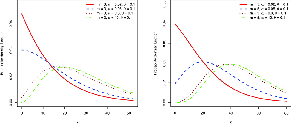

Close

Fig. 1

The PDF of $\mathit{AA}(m,\alpha ,\theta )$ for some values of parameters.

Export to PPT

Close

Fig. 2

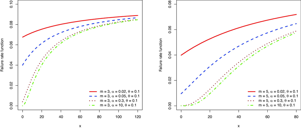
The failure rate function of $\mathit{AA}(m,\alpha ,\theta )$ for some values of parameters.

Export to PPT

Close

Fig. 3

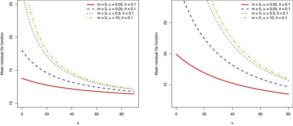
The mean residual life of $\mathit{AA}(m,\alpha ,\theta )$ for some values of parameters.

Export to PPT

Close

Fig. 4

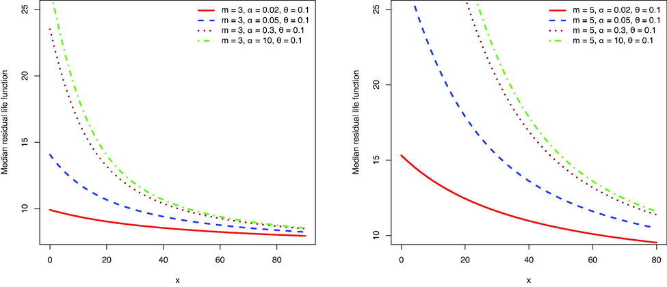
The median residual life of $\mathit{AA}(m,\alpha ,\theta )$ for some values of parameters.

Export to PPT

The mean inactivity time (MIT) at time $x,m^{\ast }\left(x\right)$ , represents the mean of elapsed time at x given the event has been occurred before x, mathematically, $$m^{\ast }\left(x\right)=E(x-X|X<x)=\frac{1}{F\left(x\right)}{\int }_0^{x}F(z)\mathit{dz},x⩾0\text{.}$$

Proposition 3

The MIT function of $\mathit{AA}(m,\alpha ,\theta )$ distribution is of the form

(16)

$$m^{\ast }\left(x\right)=(x+\frac{1}{\alpha }-\frac{1}{\theta })-\frac{1}{\theta }{e}^{-\frac{\theta }{\alpha }}\frac{{\left(\frac{\theta }{\alpha }\right)}^m-{(\frac{\theta }{\alpha }+\theta x)}^m{e}^{-\theta x}}{\mathrm{\Gamma }(\frac{\theta }{\alpha },m)-\mathrm{\Gamma }(\frac{\theta }{\alpha }+\theta x,m)},x⩾0\text{.}$$

Proof

We have

(17)

$$\begin{array}{cc}{\int }_0^{x}F\left(z\right)\mathit{dz}\hfill & =\frac{1}{\mathrm{\Gamma }(\frac{\theta }{\alpha },m)}{\int }_0^x\mathrm{\Gamma }(\frac{\theta }{\alpha },m)-\mathrm{\Gamma }(\frac{\theta }{\alpha }+\theta z,m)\mathit{dz}\hfill \\ \hfill & =\frac{1}{\mathrm{\Gamma }(\frac{\theta }{\alpha },m)}\left(x\mathrm{\Gamma }(\frac{\theta }{\alpha },m)-{\int }_0^x\mathrm{\Gamma }(\frac{\theta }{\alpha }+\theta z,m)\mathit{dz}\right)\text{.}\hfill \end{array}$$

Now, we can simplify the integral in the last expression as follows.

(18)

$$\begin{array}{cc}\hfill & {\int }_0^x\mathrm{\Gamma }(\frac{\theta }{\alpha }+\theta z,m)\mathit{dz}={\int }_0^x{\int }_{\frac{\theta }{\alpha }+\theta z}^{\infty }{t}^{m-1}{e}^{-t}\mathit{dtdz}\hfill \\ \hfill & ={\int }_{\frac{\theta }{\alpha }}^{\frac{\theta }{\alpha }+\theta x}{\int }_0^{\frac{t}{\theta }-\frac{1}{\alpha }}{t}^{m-1}{e}^{-t}\mathit{dzdt}+{\int }_{\frac{\theta }{\alpha }+\theta x}^{\infty }{\int }_0^x{t}^{m-1}{e}^{-t}\mathit{dzdt}\hfill \\ \hfill & =\frac{1}{\theta }\left(\mathrm{\Gamma }(\frac{\theta }{\alpha },m+1)-\mathrm{\Gamma }(\frac{\theta }{\alpha }+\theta x,m+1)\right)-\frac{1}{\alpha }\left(\mathrm{\Gamma }(\frac{\theta }{\alpha },m)-\mathrm{\Gamma }(\frac{\theta }{\alpha }+\theta x,m)\right)+x\mathrm{\Gamma }(\frac{\theta }{\alpha }+\theta x,m)\text{.}\hfill \end{array}$$

On the other hand

(19)

$$\begin{array}{cc}\mathrm{\Gamma }(\frac{\theta }{\alpha },m+1)-\mathrm{\Gamma }(\frac{\theta }{\alpha }+\theta x,m+1)\hfill & =m\mathrm{\Gamma }(\frac{\theta }{\alpha },m)+{\left(\frac{\theta }{\alpha }\right)}^m{e}^{-\frac{\theta }{\alpha }}\hfill \\ \hfill & -m\mathrm{\Gamma }(\frac{\theta }{\alpha }+\theta x,m)-{(\frac{\theta }{\alpha }+\theta x)}^m{e}^{-(\frac{\theta }{\alpha }+\theta x)}\text{.}\hfill \end{array}$$

Then, the results follows by (17), (18) and (19). □

The quantile inactivity time is an alternative for MIT and represents, at time x, the quantile of the elapsed time given the event occurred before x. For a distribution F, it is defined by:

(20)

$$q_p^{\ast }\left(x\right)=x-F^{-1}\left(\overline{p}F\right(x\left)\right),x⩾0\text{.}$$ and for $\mathit{AA}(m,\alpha ,\theta )$ can be written as

(21)

$$q_p^{\ast }\left(x\right)=x-\frac{1}{\theta }{\mathrm{\Gamma }}^{-1}\left(p\mathrm{\Gamma }\left(\frac{\theta }{\alpha },m\right)+\overline{p}\mathrm{\Gamma }\left(\frac{\theta }{\alpha }+\theta x,m\right),m\right)+\frac{1}{\alpha },x⩾0\text{.}$$

Fig. 5 shows the MIT and the median inactivity time ( $q_{0.5}^{\ast }\left(x\right)$ ) of $\mathit{AA}(m,\alpha ,\theta )$ for some parameters and shows increasing and convex forms. The greater values of the MIT indicate that the conditional distribution of the elapsed time is skewed to right.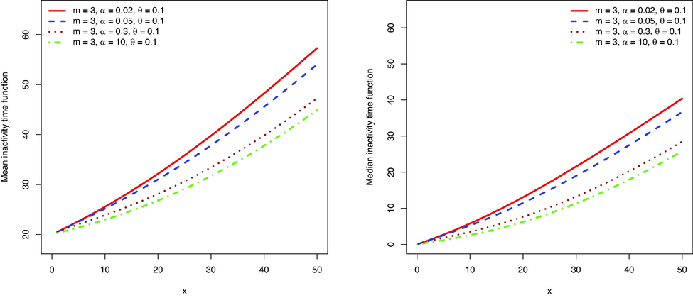

Close

Fig. 5

Left: The MIT of $\mathit{AA}(m,\alpha ,\theta )$ for some values of the parameters. Right: The median inactivity time of this distribution for the selected values of the parameters.

Export to PPT

4 Estimation of the parameters

Let m be known. By the moments method and applying (9), we can estimate $(\alpha ,\theta )$ by minimizing the following expression. $$\mathrm{\Delta }(\alpha ,\theta )={(\bar{X}-E(X\left)\right)}^2+{(\overline{X^2}-E(X^2\left)\right)}^2\text{.}$$

So, the moments estimator is $$(\widehat{\alpha },\widehat{\theta })=\arg {\displaystyle \underset{\alpha ,\theta }{\min }}\mathrm{\Delta }(\alpha ,\theta )\text{.}$$

The moment estimates can be used as initial values for maximizing the log-likelihood function and finding the maximum likelihood estimator (MLE).

Let m be known and $x_1,x_2,\dots ,x_n$ represents a realization from $\mathit{AA}(m,\alpha ,\theta )$ , the log-likelihood function is $$l(\alpha ,\theta \text{;}\mathbf{x})=-n\frac{\theta }{\alpha }+\mathit{nm}\ln \theta -n(m-1)\ln \alpha -n\ln \mathrm{\Gamma }(\frac{\theta }{\alpha },m)+{\displaystyle \sum _{i=1}^n}(m-1)\ln (1+\alpha x_i)-\theta {\displaystyle \sum _{i=1}^n}{x}_i\text{.}$$

Also, the likelihood equations are as follows: $$\frac{\partial l}{\partial \alpha }=n\frac{\theta }{{\alpha }^2}-n\frac{m-1}{\alpha }-n\frac{{\left(\frac{\theta }{\alpha }\right)}^m{e}^{-\frac{\theta }{\alpha }}}{\alpha \mathrm{\Gamma }(\frac{\theta }{\alpha },m)}+(m-1){\displaystyle \sum _{i=1}^n}\frac{x_i}{1+\alpha x_i}=0,$$ and $$\frac{\partial l}{\partial \theta }=-\frac{n}{\alpha }+\frac{\mathit{nm}}{\theta }+n\frac{{\left(\frac{\theta }{\alpha }\right)}^{m-1}{e}^{-\frac{\theta }{\alpha }}}{\alpha \mathrm{\Gamma }(\frac{\theta }{\alpha },m)}-{\displaystyle \sum _{i=1}^n}{x}_i=0\text{.}$$

The MLE can be calculated by maximizing the log-likelihood function or by solving the likelihood equations. If m is not known, which is usually the case, we can estimate the parameters for a range of m values and then choose the best model based on the Kolmogorov–Smirnov (K-S) statistic or other criteria.

The Fisher information matrix for the $\mathit{AA}(m,\alpha ,\theta )$ is of the form $$K=\left[\begin{array}{cc}E\left(-\frac{{\partial }^{2}l}{\partial {\alpha }^2}\right)\hfill & E\left(-\frac{{\partial }^{2}l}{\partial \alpha \partial \theta }\right)\hfill \\ E\left(-\frac{{\partial }^{2}l}{\partial \theta \partial \alpha }\right)\hfill & E\left(-\frac{{\partial }^{2}l}{\partial {\theta }^2}\right)\hfill \end{array}\right]\text{.}$$ where Let $l=\ln f\left(X\right)$ . Let $X_i,i=1,2,\dots ,n$ stands for a sample from $\mathit{AA}(m,{\alpha }_0,{\theta }_0)$ . Then, the MLE, $(\widehat{\alpha },\widehat{\theta })$ , converges in distribution to bivariate normal $N\left(\right({\alpha }_0,{\theta }_0),n^{-1}{K}^{-1})$ in which $K^{-1}$ is the inverse of the information matrix.

Suppose that events are subject to random right censorship. A random event $X_i$ is said to be right-censored if the only information about the event is that it is greater than the random censoring variable $C_i$ , i.e. $X_i>C_i$ . So, the observations of a right censored random sample consist of $T_i=\min (X_i,C_i)$ and $d_i$ , where $d_i=1$ if the event is not censored, $X_i⩽C_i$ , and $d_i=0$ if the event is censored, $X_i>C_i$ . Let we have one right censored sample $(t_i,d_i),i=1,2,\dots ,n$ . Then, the log-likelihood function is $$l(\alpha ,\theta \text{;}\mathbf{t},\mathbf{d})={\displaystyle \sum _{i=1}^n}{d}_i\ln f\left(t_i\right)+{\displaystyle \sum _{i=1}^n}(1-d_i)\ln R\left(t_i\right)\text{.}$$ in which f and R are the PDF and the reliability functions of the $\mathit{AA}(m,\alpha ,\theta )$ respectively. It is easy to check that the log-likelihood function simplifies to $$\begin{array}{cc}l(\alpha ,\theta \text{;}\mathbf{t},\mathbf{d})\hfill & =n\ln \mathrm{\Gamma }\left(\frac{\theta }{\alpha },m\right)+{\displaystyle \sum _{i=1}^n}{d}_i\left(-\frac{\theta }{\alpha }+m\ln \theta -(m-1)\ln \alpha +(m-1)\ln (1+\alpha t_i)-\theta t_i\right)\hfill \\ \hfill & +{\displaystyle \sum _{i=1}^n}(1-d_i)\ln \mathrm{\Gamma }\left(\frac{\theta }{\alpha }+\theta t_i,m\right)\text{.}\hfill \end{array}$$

5 Simulation

Given that $\mathit{AA}(m,\alpha ,\theta )$ is a mixture of gamma distributions, we can extract a random sample of size n from this model as described in the following steps:

1. Simulate one random instance of multinomial distribution with parameters $n,w_1,w_2$ ,…, $w_m$ , where $w_i$ is defined by (3). Let the simulated instance be $(n_1,n_2,\dots ,n_m)$ which will satisfy $n_1+n_2+\dots +n_m=n$ .

2. For every $n_i$ , simulate one random sample of the gamma distribution $G(m-i+1,\theta )$ of size $n_i$ . Then combine these samples to provide one sample of size n from $\mathit{AA}(m,\alpha ,\theta )$ .

3. Here, the degenerate random variable with mean $t_{\ast }$ has been used as the random censorship variable $C_i$ . Given the censorship percentage p, we have $t_{\ast }=q\left(\overline{p}\right)$ where $q\left(\right)$ is defined in (11).

The simulation results have been abstracted in Table 1. We have considered two values $p=0$ and $0.2$ for censorship rate. Every cell of the table shows the results for one run. In every run, we provide $r=1000$ replicates of samples of size $n=80,100$ . For every sample the MLE, $(\widehat{\alpha },\widehat{\theta })$ has been computed. Then the bias (B), absolute bias (AB) and the mean squared error (MSE) for both $\alpha$ and $\theta$ have been computed. These measures are defined in the following relations for $\alpha$ . They are defined similarly for $\theta$ . $$B_{\alpha }=\frac{1}{r}{\displaystyle \sum _{i=1}^r}({\widehat{\alpha }}_i-\alpha ),$$ $${\mathit{AB}}_{\alpha }=\frac{1}{r}{\displaystyle \sum _{i=1}^r}|{\widehat{\alpha }}_i-\alpha |,$$ and $${\mathit{MSE}}_{\alpha }=\frac{1}{r}{\displaystyle \sum _{i=1}^r}{({\widehat{\alpha }}_i-\alpha )}^2\text{.}$$

Some of the main observations from simulation results are listed in the following.

• The MLE of the parameters are consistent, i.e., AB and MSE decrease with n.

• The AB and MSE have larger values for censored data ( $p=0.2$ ) rather than uncensored data.

6 Applications

Shanker (2016a,b) analyzed a data set consisting of the number of cycles to failure for 25 yarn samples. The data are: 15, 20, 38, 42, 61, 76, 86, 98, 121, 146, 149, 157, 175, 176, 180, 180, 198, 220, 224, 251, 264, 282, 321, 325, 653. The MLE of the parameters of $\mathit{AA}(m,\alpha ,\theta )$ was calculated from $m=1,2,\dots ,20$ . For $m=10$ , we have the smallest value of the K-S statistic. Thus, the estimated model is $\mathit{AA}(10,0.003368,0.022551)$ . The K-S statistic and corresponding p-value are $0.105787$ and $0.942375$ , respectively. The AIC value, which corresponds to the MLE, is $306.2316$ . Fig. 6, left panel, shows the empirical CDF and the CDF of the fitted model, and graphically confirms that the model describes the data well. Also, Fig. 8, left panel, draws the histogram of data and the estimated PDFs.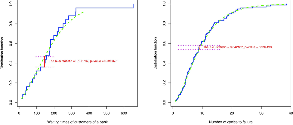

Close

Fig. 6

The empirical distribution function along with fitted $\mathit{AA}(m,\alpha ,\theta )$ .

Export to PPT

Close

Fig. 8

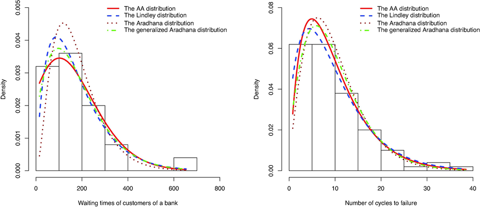
The histogram along with some fitted models for the first data set (left) and the second data set (right).

Export to PPT

The second data set consist of 100 waiting times (in minutes) of customers to be served in a bank: 0.8, 0.8, 1.3, 1.5, 1.8, 1.9, 1.9, 2.1, 2.6, 2.7, 2.9, 3.1, 3.2, 3.3, 3.5, 3.6, 4.0, 4.1, 4.2, 4.2, 4.3, 4.3, 4.4, 4.4, 4.6, 4.7, 4.7, 4.8, 4.9, 4.9, 5.0, 5.3, 5.5, 5.7, 5.7, 6.1, 6.2, 6.2, 6.2, 6.3, 6.7, 6.9, 7.1, 7.1, 7.1, 7.1, 7.4, 7.6, 7.7, 8.0, 8.2, 8.6, 8.6, 8.6, 8.8, 8.8, 8.9, 8.9, 9.5, 9.6, 9.7, 9.8, 10.7, 10.9, 11.0, 11.0, 11.1, 11.2, 11.2, 11.5, 11.9, 12.4, 12.5, 12.9, 13.0, 13.1, 13.3, 13.6, 13.7, 13.9, 14.1, 15.4, 15.4, 17.3, 17.3, 18.1, 18.2, 18.4, 18.9, 19.0, 19.9, 20.6, 21.3, 21.4, 21.9, 23.0, 27.0, 31.6, 33.1, 38.5, see Ghitany et al. (2008) and Shanker (2015).

For $m=1,2,\dots ,20$ , the MLEs of the parameters of $\mathit{AA}(m,\alpha ,\theta )$ were calculated. Based on the K-S statistics, the best model among them is $\mathit{AA}(2,1545.077,0.202477)$ . The corresponding AIC value is $638.6034$ , and the K-S statistics and p-value are $0.042187$ and $0.994198$ , respectively, indicating a good fit. Fig. 6, right panel, shows the empirical and fitted CDFs and confirms a good fit.

In a comparative analysis, we fitted the Lindley distribution, the Aradhana distribution, and the generalized Aradhana distribution defined by (1) to these data sets. The MLEs of the parameters of the models were estimated and the results, summarized in Table 2, show that the proposed model $\mathit{AA}(m,\alpha ,\theta )$ performs better than the others in both examples. Figs. 7 and 8 show the fitted distributions and PDFs respectively.

Close

Fig. 7

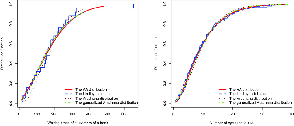
The empirical distribution function along with some fitted models for the first data set (left) and the second data set (right).

Export to PPT

7 Conclusion

Because of its applicability and usefulness, the Lindley model and its generalizations have been considered by many authors. Here, a new generalization of the Lindley distribution has been introduced to extend this collection. Some properties of this distribution have been studied. Parameter estimation was discussed using moments and maximum likelihood methods. Simulation studies show that the MLE is efficient and consistent for both complete and right-censored data. The results of fitting the presented model to two real data sets show that it is useful in analyzing data.

References

- A new generalized Lindley distribution. J. Stat. Comput. Simul.. 2015;85:3662-3678.
- [Google Scholar]
- A New Flexible Generalized Lindley Model: Properties, Estimation and Applications. Symmetry. 2020;12:1678. URL: https://www.mdpi.com/2073-8994/12/10/1678
- Al-Babtain A.A., Eid, H.A., A-Hadi N.A., Merovci, F., 2014. The five parameter Lindley distribution. Pakistan J. Stat. 31, 363–384.
- Inferences on stress-strength reliability from Lindley distribution. Commun. Stat. Theory Methods. 2013;42:1443-1463.
- A new condition for identifiability of finite mixture distributions. Metrika. 2006;63:215-221.
- [CrossRef] [Google Scholar]
- Bader, M.G., Priest, A.M., 1982. Statistical aspects of fiber and bundle strength in hybrid composites. In hayashi, T., Kawata, K. Umekawa, S. (Eds), Progress in Science in engineering Composites, ICCM-IV, Tokyo. 1129–1136.
- The Lindley family of distributions: properties an applications. Hacettepe J. Math. Stat.. 2017;46:1113-1137.
- The Lindley Weibull Distribution: properties and applications. Acad. Bras. Cienc.. 2018;90(3):2579-2598. PMID:30304208
- Fracture mechanics approach to the design of glass aircraft windows: A case study. SPIE Proc.. 1994;2286:419-430.
- A two-parameter Lindley distribution and its applications to survival data. Math. Comput. Simul.. 2011;81:1190-1201.
- Survival Distributions: Reliability Applications in the Biometrical Sciences. New York: John Wiley; 1976.
- Mixture models: theory, geometry and applications. In: NSF-CBMS Regional Conference Series in Probability and Statistics. 1995. p. :5.
- Families of frequency distributions. London, U.K.: Charles Griffin; 1972.
- On Generalized Lindley Distribution and Its Applications to Model Lifetime Data from Biomedical Science and Engineering. Insights Biomed.. 2016;1(2)
- A two-parameter power Aradhana distribution with properties and application. Indian J. Ind. Appl. Math.. 2018;9:210-220.
- Statistical analysis of finite mixture distributions. Chichester, U.K.: John Wiley and Sons; 1985.
- A generalized Aradhana distribution with properties and applications. Biometrics Biostat. Int. J.. 2018;7(4):374-385.