A new extended Rayleigh distribution

Abdulhakim A. Al-Babtain

doi:10.1016/j.jksus.2020.04.015

View/Download PDF

Buy Reprints

PDF

Translate this page into:

Original article

32 (

); 2576-2581

doi:

10.1016/j.jksus.2020.04.015

A new extended Rayleigh distribution

Abdulhakim A. Al-Babtain

Department of Statistics and Operations Research, King Saud University, Saudi Arabia

Received: 2019-11-5, Accepted: 2020-4-18, Published: 2020-07-01

Disclaimer:
This article was originally published by Elsevier and was migrated to Scientific Scholar after the change of Publisher.

Peer review under responsibility of King Saud University.

Abstract

In this paper, we proposed a new extension of the Rayleigh distribution with two parameter called type I half logistic Rayleigh distribution. Several important mathematical and statistical properties of this new distribution are discussed. Simulation studies and real data applications are also considered for performance of the new distribution.

Keywords

Rayleigh distribution

type I half logistic distribution

Moments

Order statistics

Maximum likelihood estimation

Simulation study

Show Related Articles from PubMed

1 Introduction

Many new statistical distributions have been derived using the commonly known distributions by way of different types of transformations or compounding. In the last few years, new generated families of continuous distributions have attracted several statisticians to develop new models. These families are obtained by introducing one or more additional shape parameter(s) to the baseline distribution. Some of the generated families are: the beta-G (Eugene et al., 2002), gamma-G (type 1) (Zografos and Balakrishnan, 2009), gamma-G (type 2) (Ristic and Balakrishnan, 2012), transformed-transformer (T-X; Alzaatreh et al., 2013), Weibull- G (Bourguignon et al., 2014), Weibull- G (Bourguignon et al., 2014), exponentiated half-logistic-G (Cordeiro et al., 2014), type I half logistic–G family (Cordeiro et al., 2015), exponentiated Weibull-G (Hassan and Elgarhy, 2016), type II half logistic – G (Hassan et al., 2017).

Based on Cordeiro et al. (2015), the cumulative distribution function (CDF) and the probability density function (PDF) of type I half logistic – G family are given by

(1)

F_{λ} (x) = \frac{1 - {[1 - G (x)]}^{λ}}{1 + {[1 - G (x)]}^{λ}} |_{x, λ, > 0},

and

(2)

f_{λ} (x) = \frac{2 λ g (x) {[1 - G (x)]}^{λ - 1}}{{\{1 + {[1 - G (x)]}^{λ}\}}^{2}} |_{x, λ, > 0},

respectively, where

λ

is the shape parameter.

Lord Rayleigh (1880) introduced the Rayleigh distribution in connection with a problem in the field of acoustics. In nature, physical phenomena in many areas of fields of science (for example, noise theory, lethality, radar return, etc.) have amplitude distributions which can be characterized by the Rayleigh density function or some function which can be derived from the Rayleigh density function. Because a literature search failed to turn up any major source of material on the Rayleigh density function.

The probability density function (PDF), cumulative distribution function (CDF), of the Rayleigh distribution are given, respectively, by

(3)

g_{α} (x) = {2 α x e}^{- α x^{2}} |_{α > 0, x > 0},

and

(4)

G_{α} (x) = {1 - e}^{- α x^{2}} |_{α > 0, x > 0},

where,

α

is the scale parameter.

In this paper we introduce a new two-parameter model as a competitive extension for Rayleigh distribution using the TIHL-G distributions. The rest of the paper is outlined as follows. In Section 2, we define the type I half-logistic Rayleigh (TIHLR) distribution. In Section 3, we derive a very useful representation for the (TIHLR) PDF and CDF functions, some mathematical properties of the proposed distribution are derived. The maximum likelihood method is applied to drive the estimates of the model parameters in Section 4. Simulation study is carried out to estimate the model parameters of (TIHLR) distribution in Section 5. Section 6 gives an illustrative example to explain how the real data sets can be modeled by TIHLR.

2 The new model

In this section, the two-parameter TIHLR distribution is obtained by substituting (3) into (1) and (4) into (2), the CDF and PDF of type I half-logistic Rayleigh distribution, takes the following form

(5)

F_{φ} (x) = \frac{1 - e^{- α λ x^{2}}}{1 + e^{- α λ x^{2}}} |_{λ, α > 0, x > 0},

and

(6)

f_{φ} (x) = \frac{4 λ α x e^{- α λ x^{2}}}{{[1 + e^{- α λ x^{2}}]}^{2}} |_{λ, α > 0, x > 0},

where,

φ = (λ, α)

is the set of parameters. The survival and hazard rate functions of TIHLR distribution are respectively given by

${\bar{F}}_{φ} (x) = \frac{2 e^{- α λ x^{2}}}{1 + e^{- α λ x^{2}}}, a n d h_{φ} (x) = \frac{2 λ α x}{1 + e^{- α λ x^{2}}} .$

The following plots show the PDF and hazard rate function of TIHLR distribution for some parameter values are displayed in Figs. 1 and 2 respectively.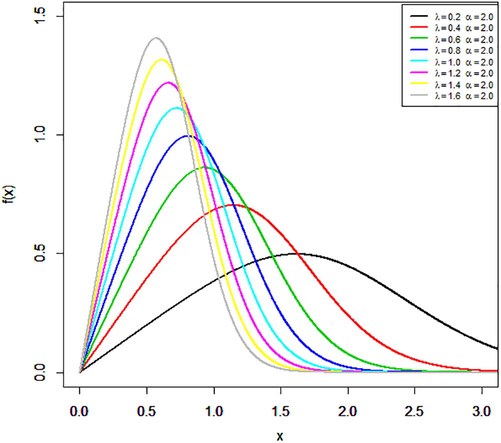

Plots of the PDF of the TIHLR distribution for some parameter values.

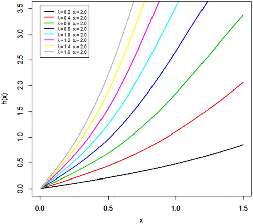
Plots of the hazard rate function of the TIHLR distribution for some parameter values.

Some important extensions of the Rayleigh model have been developed and studied such as Yousof et al. (2015, 2016); Korkmaz et al. (2017, 2018, 2019); Brito et al. (2017); Hamedani et al. (2017); Cordeiro et al. (2018); Yousof et al. (2018a,b); Chakraborty et al. (2018); Hamedani et al. (2018, 2019) among others.

3 Statistical properties

In this section some properties of the TIHLR distribution are obtained.

3.1

3.1 Useful expansions

In this subsection representations of the PDF and CDF for TIHLR distribution are derived.

Using the generalized binomial expansion for β > 0 and |Z| > 1

(7)

{(1 + z)}^{- β} = \sum_{k = 0}^{\infty} {(- 1)}^{k} (\binom{β + k - 1}{k}) z^{k},

the distribution function of TIHLR distribution becomes

(8)

f_{φ} (x) = \sum_{k = 0}^{\infty} η_{k} x e^{- α λ (k + 1) x^{2}},

where $η_{k} = {4 λ α (- 1)}^{k} (\binom{β + k - 1}{k}) .$

3.2

3.2 Quantile and median

Quantile functions are used in theoretical aspects of probability theory, statistical applications and simulations. Simulation methods utilize quantile function to produce simulated random variables for classical and new continuous distributions. The quantile function, say Q(u) = $F^{- 1} (u)$ of X is given by $u = \frac{1 - e^{- α λ {(Q (u))}^{2}}}{1 + e^{- α λ {(Q (u))}^{2}}},$ after some simplifications, it reduces to the following form

(9)

Q (u) = \sqrt{\frac{1}{α λ} \ln (\frac{1 + u}{1 - u})} .

where,

u

is considered as a uniform random variable on the unit interval (0,1).

In particular, the median can be derived from (9) be setting u = 0.5. Then, the median is given by $median = \sqrt{\frac{1}{α λ} \ln (3)}$

3.3

3.3 Moments

If X has the PDF (6), then its rth moment can be obtained through the following relation

(10)

{\overset{`}{μ}}_{r} = E (X^{r}) = \int_{0}^{\infty} x^{r} f (x) d x .

Substituting (8) into (10) yields ${\overset{`}{μ}}_{r} = \sum_{k = 0}^{\infty} η_{k} \int_{0}^{\infty} x^{r + 1} e^{- α λ (k + 1) x^{2}} d x .$

Then, ${\overset{`}{μ}}_{r} = \sum_{k = 0}^{\infty} \frac{η_{k}}{2 {[α λ (k + 1)]}^{\frac{r}{2} + 1}} Γ (\frac{r}{2} + 1) .$ and the moment generating function of TIHLR distribution is obtained through the following relation $M_{X} (t) = \sum_{r = 0}^{\infty} \frac{t^{r}}{r!} E (X^{r}) = \sum_{k, r = 0}^{\infty} \frac{t^{r} η_{k}}{2 r! {[α λ (k + 1)]}^{\frac{r}{2} + 1}} Γ (\frac{r}{2} + 1) .$

Also, the incomplete moment, say $φ_{s} (t)$ , is given by $φ_{s} (t) = \underset{0}{\int^{t}} x^{s} f (x) d x .$

Using (6), then $φ_{s} (t)$ can written as follows $φ_{s} (t) = \sum_{k = 0}^{\infty} η_{k} \int_{0}^{t} x^{s + 1} e^{- α λ (k + 1) x^{2}} d x .$

Then, using the lower incomplete gamma function, we obtain

(11)

φ_{s} (t) = \sum_{k = 0}^{\infty} \frac{η_{k}}{2 {[α λ (k + 1)]}^{\frac{s}{2} + 1}} γ (\frac{s}{2} + 1, α λ (k + 1) t^{2}),

where

Y (s, t) = \underset{0}{\int^{t}} x^{s - 1} e^{- x} d x,

is the lower incomplete gamma function. Further, the conditional moments, say

τ_{s} (t)

, is given by

τ_{s} (t) = \underset{t}{\int^{\infty}} x^{s} f (x) d x = \sum_{k = 0}^{\infty} η_{k} \int_{t}^{\infty} x^{s + 1} e^{- α λ (k + 1) x^{2}} d x,

then we get the following

τ_{s} (t) = \sum_{k = 0}^{\infty} \frac{η_{k}}{2 {[α λ (k + 1)]}^{\frac{s}{2} + 1}} Γ (\frac{s}{2} + 1, α λ (k + 1) t^{2}),

where

Γ (s, t) = \underset{t}{\int^{\infty}} x^{s - 1} e^{- x} d x

is the upper incomplete gamma function.

3.4

3.4 Residual life function

The nth moment of the residual life of X is given by $m_{n} (t) = \frac{1}{R (t)} \underset{t}{\int^{\infty}} {(x - t)}^{n} f (x) d x .$

Applying the binomial expansion of ${(x - t)}^{n}$ into the above formula, we get

(12)

m_{n} (t) = \frac{1}{R (t)} \sum_{k = 0}^{\infty} \sum_{d = 0}^{n} {(- t)}^{d} (\binom{n}{d}) \frac{η_{k}}{2 {[α λ (k + 1)]}^{\frac{n - d}{2} + 1}} Γ (\frac{n - d}{2} + 1, α λ (k + 1) t^{2}) .

3.5

3.5 Simple type Copula-based construction

We will consider several Copula approaches to construct the bivariate and the multivariate TIHLR type distributions via copula (or with straightforward bivariate CDFs form, in which we just need to consider two different TIHLR CDFs).

3.5.1

3.5.1 The bivariate TIHLR extension using the Morgenstern family

First, we start with CDF for Morgenstern family of two RVs $(Y_{1}, Y_{2})$ which has the following form $F_{c} (y_{1}, y_{2}) |_{(| λ | \leq 1)} = F_{1} (y_{1}) F_{2} (y_{2}) \{1 + c [1 - F_{1} (y_{1})] [1 - F_{2} (y_{2})]\},$

Setting ${F_{1} (y_{1}) = F}_{α_{1}, λ_{1}} (y_{1}) = \frac{1 - e^{- α_{1} λ_{1} {y_{1}}^{2}}}{1 + e^{- α_{1} λ_{1} {y_{1}}^{2}}},$

and ${F_{2} (y_{2}) = F}_{α_{2}, λ_{2}} (y_{2}) = \frac{1 - e^{- α_{2} λ_{2} {y_{2}}^{2}}}{1 + e^{- α_{2} λ_{2} {y_{2}}^{2}}},$

then we have a 5-dimension parameter model as $F_{λ} (y_{1}, y_{2}) |_{(|λ| \leq 1)} = \frac{1 - e^{- α_{1} λ_{1} {y_{1}}^{2}}}{1 + e^{- α_{1} λ_{1} {y_{1}}^{2}}} \times \frac{1 - e^{- α_{2} λ_{2} {y_{2}}^{2}}}{1 + e^{- α_{2} λ_{2} {y_{2}}^{2}}} \times \{1 + λ [(1 - \frac{1 - e^{- α_{1} λ_{1} {y_{1}}^{2}}}{1 + e^{- α_{1} λ_{1} {y_{1}}^{2}}}) (1 - \frac{1 - e^{- α_{2} λ_{2} {y_{2}}^{2}}}{1 + e^{- α_{2} λ_{2} {y_{2}}^{2}}})]\} .$

3.5.2

3.5.2 Via clayton copula

3.5.2.1

3.5.2.1 The bivariate TIHLR extension

The bivariate extension via clayton copula can be considered as a weighted version of the clayton copula, which is of the form $C (u, v) = {[u^{- (δ_{1} + δ_{2})} + v^{- (δ_{1} + δ_{2})} - 1]}^{- \frac{1}{δ_{1} + δ_{2}}} .$

This is indeed a valid copula. Next, let us assume that X ∼ TIHLR $(α_{1}, λ_{1})$ and X ∼ TIHLR $(α_{2}, λ_{2}) .$ Then, setting $u = u_{α_{1}, λ_{1}} (x) = \frac{1 - e^{- α_{1} λ_{1} x^{2}}}{1 + e^{- α_{1} λ_{1} x^{2}}}$ and $v = v_{α_{2}, λ_{2}} (y) = \frac{1 - e^{- α_{2} λ_{2} y^{2}}}{1 + e^{- α_{2} λ_{2} y^{2}}},$ the associated CDF bivariate TIHLR type distribution is $H (x, y) = {[{(\frac{1 - e^{- α_{1} λ_{1} x^{2}}}{1 + e^{- α_{1} λ_{1} x^{2}}})}^{- (δ_{1} + δ_{2})} + {(\frac{1 - e^{- α_{2} λ_{2} y^{2}}}{1 + e^{- α_{2} λ_{2} y^{2}}})}^{- (δ_{1} + δ_{2})} - 1]}^{- \frac{1}{δ_{1} + δ_{2}}} .$

Note: Depending on the specific baseline CDF, one may construct various bivariate TIHLR type model in which $(δ_{1} + δ_{2}) \geq 0 .$

3.5.2.2

3.5.2.2 The Multivariate TIHLR extension

The $d$ -dimensional version from the above is $H (y_{1}, y_{2}, \dots, y_{d}) = {\{\sum_{i = 1}^{d} {\{\frac{1 - e^{- α_{i} λ_{i} {y_{i}}^{2}}}{1 + e^{- α_{i} λ_{i} {y_{i}}^{2}}}\}}^{- (δ_{1} + δ_{2})} + 1 - d\}}^{- 1 / (δ_{1} + δ_{2})} .$

Further future works could be allocated for studying the bivariate and the multivariate extensions of the TIHLR model.

4 Maximum likelihood estimation

The maximum likelihood estimates (MLEs) of the unknown parameters for the TIHLR distribution are determined based on complete samples. Let $X_{1}, X_{2}, \dots X_{n}$ be observed values from the TIHLR distribution with set of parameters $φ = {(λ, α)}^{T}$ The log-likelihood function for the vector of parameters $φ$ can be expressed as $\ln L (φ) = n \ln (4 λ) + n \ln (α) + n \ln (β) + \sum_{i = 1}^{n} {l n (x}_{i}) - α λ \sum_{i = 1}^{n} {x^{2}}_{i} - 2 \sum_{i = 1}^{n} \ln (1 + e^{- α λ {x^{2}}_{i}}) .$

The elements of the score function $U (φ) = (U_{λ}, U_{α})$ are given by $U_{λ} = \frac{n}{λ} - α \sum_{i = 1}^{n} {x^{2}}_{i} + 2 α \sum_{i = 1}^{n} \frac{{x^{2}}_{i} e^{- α λ {x^{2}}_{i}}}{1 + e^{- α λ {x^{2}}_{i}}},$ and $U_{α} = \frac{n}{α} - λ \sum_{i = 1}^{n} {x^{2}}_{i} + 2 λ \sum_{i = 1}^{n} \frac{{x^{2}}_{i} e^{- α λ {x^{2}}_{i}}}{1 + e^{- α λ {x^{2}}_{i}}} .$

Then the maximum likelihood estimates of the parameters λ and α are obtained by setting the last two equations to be zero and solving them. Clearly, it is difficult to solve them, therefore applying the Newton-Raphson’s iteration method and using the computer package such as Maple or R or other software.

5 Simulation study

It is very difficult to compare the theoretical performances of the different estimators (MLE) for the TIHLR distribution. Therefore, simulation is needed to compare the performances of the different methods of estimation mainly with respect to their biases, mean square errors and Variances (MLEs) for different sample sizes. A numerical study is performed using Mathematica 9 software. Different sample sizes are considered through the experiments at size n = 50, 100, 150, 200 and 300. In addition, the different values of parameters λ and α. The experiment will be repeated 10,000 times. In each experiment, the estimates of the parameters will be obtained by maximum likelihood methods of estimation. The means, MSEs and biases for the different estimators will be reported from these experiments (see Table 1).

Table 1 The parameter estimation from TIHLR distribution using MLE.

n	Par	Init	MLE	Bais	MSE	Init	MLE	Bais	MSE
50	λ	0.4	0.5158	0.0158	0.0087	1.5	0.5146	0.0146	0.0082
50	α	0.5	0.4126	0.0126	0.0055	0.5	1.5439	0.0439	0.0741

100	λ	0.4	0.5066	0.0066	0.0039	1.5	0.5075	0.0075	0.0038
100	α	0.5	0.4053	0.0053	0.0025	0.5	1.5225	0.0225	0.0343

150	λ	0.4	0.5052	0.0052	0.0024	1.5	0.5049	0.0049	0.0026
150	α	0.5	0.4041	0.0041	0.0016	0.5	1.5147	0.0147	0.0231

200	λ	0.4	0.5035	0.0035	0.0019	1.5	0.5031	0.0031	0.0019
200	α	0.5	0.4028	0.0028	0.0012	0.5	1.5093	0.0093	0.0169

300	λ	0.4	0.5028	0.0028	0.0012	1.5	0.5025	0.0025	0.0012
300	α	0.5	0.4022	0.0022	0.0008	0.5	1.5076	0.0076	0.0110

50	λ	2	0.5147	0.0147	0.0086	2.5	0.5147	0.0147	0.0085
50	α	0.5	2.0587	0.0587	0.1374	0.5	2.5735	0.0735	0.2117

100	λ	2	0.5078	0.0078	0.0040	2.5	0.5081	0.0081	0.0040
100	α	0.5	2.0312	0.0312	0.0647	0.5	2.5403	0.0403	0.1001

150	λ	2	0.5043	0.0043	0.0025	2.5	0.5052	0.0052	0.0025
150	α	0.5	2.0174	0.0174	0.0403	0.5	2.5261	0.0261	0.0630

200	λ	2	0.5035	0.0035	0.0019	2.5	0.5038	0.0038	0.0019
200	α	0.5	2.0139	0.0139	0.0304	0.5	2.5192	0.0192	0.0471

300	λ	2	0.5026	0.0026	0.0012	2.5	0.5024	0.0024	0.0012
300	α	0.5	2.0102	0.0102	0.0194	0.5	2.5120	0.0120	0.0311

50	λ	3	2.0621	0.0621	0.1350	5	2.0581	0.0581	0.1354
50	α	2	3.0932	0.0932	0.3038	2	5.1452	0.1452	0.8461

100	λ	3	2.0304	0.0304	0.0616	5	2.0302	0.0302	0.0623
100	α	2	3.0456	0.0456	0.1385	2	5.0754	0.0754	0.3896

150	λ	3	2.0202	0.0202	0.0409	5	2.0184	0.0184	0.0401
150	α	2	3.0303	0.0303	0.0919	2	5.0461	0.0461	0.2507

200	λ	3	2.0137	0.0137	0.0297	5	2.0144	0.0144	0.0293
200	α	2	3.0206	0.0206	0.0668	2	5.0360	0.0359	0.1833

300	λ	3	2.0091	0.0091	0.0190	5	2.0090	0.0090	0.0196
300	α	2	3.0137	0.0137	0.0428	2	5.0226	0.0226	0.1224

6 Data analysis

In this section, we use one real data set to illustrate the importance and flexibility of the TIIHLR distribution. We compare the fit of the TIHLR model with Rayleigh (R) distribution.

The Akaike information criterion (AIC), the corrected Akaike information criterion (CAIC), Bayesian information criterion (BIC), Hannan-Quinn information criterion (HQIC), Anderson-Darling (A*) and Cramér-Von Mises (W*) statistics are used for model selection.

The data set (gauge lengths of 10 mm) from Kundu and Raqab (2009). This data set consists of, 63 observations: 1.901, 2.132, 2.203, 2.228, 2.257, 2.350, 2.361, 2.396, 2.397, 2.445, 2.454, 2.474, 2.518, 2.522, 2.525, 2.532, 2.575, 2.614, 2.616, 2.618, 2.624, 2.659, 2.675, 2.738, 2.740, 2.856, 2.917, 2.928, 2.937, 2.937, 2.977, 2.996, 3.030, 3.125, 3.139, 3.145, 3.220, 3.223, 3.235, 3.243, 3.264, 3.272, 3.294, 3.332, 3.346, 3.377, 3.408, 3.435, 3.493, 3.501, 3.537, 3.554, 3.562, 3.628, 3.852, 3.871, 3.886, 3.971, 4.024, 4.027, 4.225, 4.395, 5.020.

Fig. 3 provide the plots of estimated cumulative and estimated PDF and CDF of the fitted models for the data set Table 2 lists the MLEs and their corresponding standard errors (SEs) of the model parameters for data set. The numerical values of the AIC, CAIC, BIC, HQIC, A* and W* statistics are listed in Table 3. We note that the TIHLR model gives the lowest values for the AIC, CAIC, BIC, HQIC, A* and W* statistics for data set among the fitted model. So, the TIHLR distribution could be fit the data better than R distribution. A density plot compares the fitted densities of the models with the empirical histogram of the observed data (Fig. 3).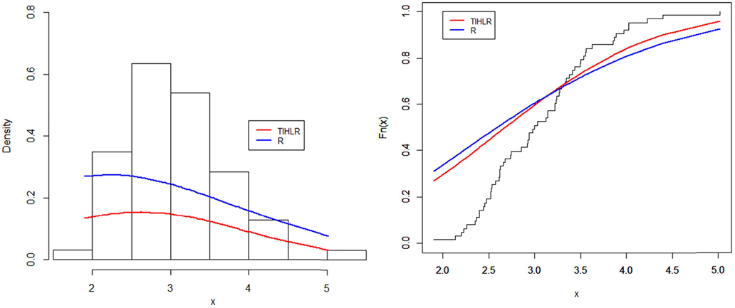

Estimates of the density and cumulative functions for the data set.

Table 2 ML estimates of the model parameters and the corresponding SEs for the data set.

Distribution	Estimated Parameters and SE
Distribution	$α$	$λ$	SE(α)	SE(λ)
TIHLR	0.029	5.267	7.024 * 10^−3	1.26449
R	0.103	–	0.0131	–

Table 3 Goodness of measures for estimates for first data set.

Model	AIC	CAIC	BIC	HQIC	A*	W*
TIHLR	173.476	173.676	173.075	175.162	18.49857	1.28789
R	189.05	189.116	188.85	189.893	32.8777	1.79986

7 Conclusion

In this paper, we propose a two-parameter model, named the TIHLR distribution. The TIHLR model is motivated by the wide use of the Rayleigh distribution in practice and also for the fact that the generalization provides more flexibility to analyze positive real-life data. We derive explicit expressions for the quantile function, ordinary moments and order statistics. The maximum likelihood estimation of the model parameters is investigated. We provide some simulation results to assess the performance of the proposed model. The practical importance of the TIIHLR distribution is demonstrated by means of one data set.

Declaration of Competing Interest

The authors declare that they have no known competing financial interests or personal relationships that could have appeared to influence the work reported in this paper.

Funding

This project supported by Researchers Supporting Project number (RSP- 2020/156) King Saud University, Riyadh, Saudi Arabia.

References

Alzaatreh A., Lee C., Famoye F.. A new method for generating families of continuous distributions. Metron. 2013;71:63-79.
[Google Scholar]
Bourguignon M., Silva R.B., Cordeiro G.M.. The Weibull– G family of probability distributions. J. Data Sci.. 2014;12:53-68.
[Google Scholar]
Brito E., Cordeiro G.M., Yousof H.M., Alizadeh M., Silva G.O.. Topp-Leone odd log-logistic family of distributions. J. Stat. Comput. Simul.. 2017;87(15):3040-3058.
[Google Scholar]
Chakraborty S., Handique L., Altun E., Yousof H.M.. A new statistical model for extreme values: mathematical properties and applications. Int. J. Open Prob. Comput. Sci. Math.. 2018;12(1):1-18.
[Google Scholar]
Cordeiro G.M., Alizadeh M., Ortega E.M.M.. The exponentiated half-logistic family of distributions: properties and applications. J. Probab. Stat. 2014 Article ID 864396, 21 pages
[CrossRef] [Google Scholar]
Cordeiro G.M., Alizadeh M., Marinho E.P.R.D.. The type I half-logistic family of distributions. J. Stat. Comput. Simul.. 2015;86:707-728.
[Google Scholar]
Cordeiro G.M., Yousof H.M., Ramires T.G., Ortega E.M.M.. The Burr XII system of densities: properties, regression model and applications. J. Stat. Comput. Simul.. 2018;88(3):432-456.
[Google Scholar]
Eugene N., Lee C., Famoye F.. The beta-normal distribution and its applications. Commun. Stat. Theory Methods. 2002;31:497-512.
[Google Scholar]
Hamedani G.G., Yousof H.M., Rasekhi M., Alizadeh M., Najibi S.M.. Type I general exponential class of distributions. Pak. J. Stat. Oper. Res.. 2017;XIV(1):39-55.
[Google Scholar]
Hamedani G.G., Altun E., Korkmaz M.C., Yousof H.M., Butt N.S.. A new extended G family of continuous distributions with mathematical properties, characterizations and regression modeling. Pak. J. Stat. Oper. Res.. 2018;14(3):737-758.
[Google Scholar]
Hamedani G.G., Rasekhi M., Najibi S.M., Yousof H.M., Alizadeh M.. Type II general exponential class of distributions. J. Stat. Oper. Res Pak 2019 forthcoming
[Google Scholar]
Hassan A.S., Elgarhy M.. A new family of exponentiated Weibull-generated distributions. Int. J. Math. Appl.. 2016;4:135-148.
[Google Scholar]
Hassan A.S., Elgarhy M., Shakil M.. Type II half Logistic family of distributions with applications. Pak. J. Stat. Oper. Res.. 2017;13(2):245-264.
[Google Scholar]
Korkmaz M.C., Yousof H.M., Ali M.M.. Some theoretical and computational aspects of the odd lindley fréchet distribution. J. Stat.: Stat. Actuarial Sci.. 2017;2:129-140.
[Google Scholar]
Korkmaz M.C., Alizadeh M., Yousof H.M., Butt N.S.. The generalized odd Weibull generated family of distributions: statistical properties and applications. Pak. J. Stat. Oper. Res.. 2018;14(3):541-556.
[Google Scholar]
Korkmaz M.C., Altun E., Yousof H.M., Hamedani G.G.. The odd power lindley generator of probability distributions: properties characterizations and regression modeling. Int. J. Stat. Prob.. 2019;8(2):70-89.
[Google Scholar]
Kundu D., Raqab M.Z.. Estimation of R= P (Y< X) for three-parameter Weibull distribution. Stat. Prob. Lett.. 2009;79:1839-1846.
[Google Scholar]
Rayleigh J.W.S.. On the resultant of a large number of vibrations of the some pitch and of arbitrary phase. Philos. Mag.. 1880;10:73-78. 5-th Series
[Google Scholar]
Ristic M.M., Balakrishnan N.. The gamma-exponentiated exponential distribution. J. Stat. Comput. Simul.. 2012;82(8):1191-1206.
[Google Scholar]
Yousof H.M., Afify A.Z., Alizadeh M., Butt N.S., Hamedani G.G., Ali M.M.. The transmuted exponentiated generalized-G family of distributions. Pak. J. Stat. Oper. Res.. 2015;11:441-464.
[Google Scholar]
Yousof H.M., Afify A.Z., Ebraheim A.N., Hamedani G.G., Butt N.S.. On six-parameter Fréchet distribution: properties and applications. Pak. J. Stat. Oper. Res.. 2016;12:281-299.
[Google Scholar]
Yousof H.M., Jahanshahi S.M., Ramires T.G., Aryal G.R., Hamedani G.G.. A new distribution for extreme values: regression model, characterizations and applications. J. Data Sci.. 2018;16(4):677-706.
[Google Scholar]
Yousof H.M., Altun E., Hamedani G.G.. A new extension of Frechet distribution with regression models, residual analysis and characterizations. J. Data Sci.. 2018;16(4):743-770.
[Google Scholar]
Zografos K., Balakrishnan N.. On families of beta- and generalized gamma-generated distributions and associated inference. Stat. Methodol.. 2009;6:344-362.
[Google Scholar]