A modified basis of cubic B-spline with free parameter for linear second order boundary value problems: Application to engineering problems

1 Introduction

There is much research that have been done on boundary value problems (BVPs) among the domains of chemistry, physics, and engineering. The standard form of second-order ODEs (Agarwal, 1986) is:

To apply an exact solution to solve physical problems is sometimes very challenging and requires extensive effort. Therefore, it is recommended to use numerical solutions for solving real-life application problems. Several numerical techniques, including the variational approach, finite difference method (FDM), finite element method (FEM), finite volume method (FVM), and the shooting method (LSM) (Fang et al., 2002; Shafie & Majid, 2012; Wang, 2009), have been applied to the two-point BVP solutions. The cubic B-spline interpolation method (CBSI) has been developed by Caglar et al. (H. Caglar et al., 2006) for two-point BVP solutions in place of the simple spline. Numerous numerical techniques based on the cubic B-splines method (CBSM) have been extensively used since then to solve both linear and nonlinear BVPs (Heilat & Hailat, 2020; Khalid et al., 2021; Tassaddiq et al., 2019). (Abd Hamid et al., 2010, 2011) investigated the cubic trigonometric B-spline and extended CBS as solutions to linear two-point BVPs. In comparison with CBSI, the trigonometric CBS produced better results. A hybrid version of the CBSM and TCBSM schemes has been created by (Heilat & Ismail, 2016) to address nonlinear two-point BVPs.

(Wasim et al., 2019) constructed an improved method to solve singular BVPs of second order by leveraging an extended cubic B-spline basis. (M. K. Iqbal et al., 2018) also have solved a variety of third-order Emden-Flower type problems with a new Cubic B-Spline approximation (NCBSA). For the solutions of non-linear higher-order Korteweg-de Vries equations, (Abbas et al., 2019) provided a new CBS approximation using the Taylor series method. (Nazir et al., 2020) investigated a novel quintic B-spline approximation and applied it to solve Boussinesq equations. (Ghaffar et al., 2019; M. Iqbal et al., 2021b; M. Iqbal et al., 2024) have also developed septic and nine-tic order splines and applied them to surfaces as tensor product schemesand have discussed the convexity of the closed shapes as 2q and ternary subdivision schemes (M. Iqbal et al., 2021a). Many authors and researchers have used higher-order numerical schemes to solve ODEs and PDEs, but these schemes have shown computationally higher costs in building the large subsequent matrix system for the solution of unknown constants (Nazir et al., 2020; Saka et al., 2022; Singh et al., 2022). Many other authors and researchers (İlhan & Şahin, 2024; Javeed & Hincal, 2024; Mulimani & Srinivasa, 2024; Nasir et al., 2023; Atta Ullah et al., 2024) have numerically solved different models of differential equations using higher-order numerical schemes. Some linear and nonlinear partial differential equations have been solved by (Khater, 2023; Atta. Ullah et al., 2023a) using the analytical and numerical schemes. (Sabir et al., 2022) discussed problems in mathematical modelling using artificial neural networks. Trigonometric and Hermite cubic splines have been used to solve the latest applications based on their ability to accurately model and interpolate complex functions, particularly in numerical solutions of differential equations (Kutluay et al., 2024; Nuri Murat and Ali Sercan, 2022; Atta. Ullah et al., 2023b; Yağmurlu & Karakaş, 2020).

Research Objective: The primary objective of this research is to enhance the smoothness of the curve solution using the modified cubic B-spline method (MCBSM) for solving linear second-order ODEs.

Problem Statement: Literatures have shown that traditional CBSM has many drawbacks when it is incorporating with the initial and boundary values (end conditions or points). This is due to the local control properties of CBSM, that affect the smoothness at near-end conditions. To address this issue, this paper proposes a modification of the basis by using a free parameter to globally control the curve solution, hence enhancing smoothness. This modification involves altering the basis of CBSM using a free parameter called $\gamma$ , in conjunction with the collocation method. The free parameter $\gamma$ gives more control over the approximation curve and consequently increases the smoothness of the curve at endpoints.

Research Advantage: The advantage of MCBSM equipped with a free parameter is that it offers a high degree of smoothness and flexibility in representing curves or surfaces, making it suitable for approximating complex functions or data sets. The modified basis can be used to approximate derivatives of ODEs.

Main Contribution and Motivation: Extensive reviews from the literatures have indicated that modifications of the basis using an extra-free parameter while maintaining the cubic order of splines have not been used to solve differential equations. This has motivated authors of this paper to explore the MCBSM as a potential solution for solving BVPs. Furthermore, convergence and error analysis of the proposed method are also investigated.

The paper is organized as follows: The definitions are discussed in Section 2. The implementation of the MCBSM and its convergence are derived in Section 3. Sections 4 and section 5 present the numerical results and the discussion, respectively. Lastly, Section 6 summarizes with a conclusion about the numerical results.

2 Derivation of MCBSM

Computer graphics, computer-aided design (CAD), and many other fields commonly use a cubic B-spline as a type of piecewise-defined curve or function when they require smooth and flexible curves. B-spline stands for “Basis spline,” and cubic B-splines are a specific type of B-spline where the basis functions are cubic polynomials. Combining these basis functions creates a continuous curve that smoothly connects a series of control points.

Consider a finite interval $[a,b]$ , where a series of equidistant partitions have been defined by breaking it down into points: $a=x_0<x_1<...<x_N=b$ . These points are evenly spaced and can express each point $x_i$ as $x_i=x_0+ih$ , where $i=0,1,2,\cdots N$ . The step size $h$ used for this partitioning is calculated as $h=\frac{(b-a)}{N}$ , where N is a positive integer.

Suppose that the proposed spline solution (Mittal & Arora, 2011) to the problem (1) is:

The first and second derivatives of equation (4) are calculated as follows:

Let $\aleph =\left\{B_{-1},B_0,B_1,\cdots ,B_{N+1}\right\}$ is a set of cubic b-spline basis and let ${\sigma }_3\left(\phi \right)=span\aleph$ . The set $\aleph$ on $[0,1]$ are linearly independent, thus ${\sigma }_3\left(\phi \right)$ has $(N+3)$ dimensions. Also, that ${\sigma }_3\left(\phi \right){\subseteq }_{\mathit{sup}}x$ .

By using equation (3), CBSM can be defined as,

Let $S\left(x\right)$ be the approximate solution of the differential equation. Then corresponding knot values for the initial and boundary conditions (endpoints) are extracted from Table 1 as shown below. $$B_0\left(x_0\right)=\frac{4}{6}=B_N\left(x_0\right),$$ $$B_{-1}\left(x_0\right)=\frac{1}{6}=B_{N-1}\left(x_0\right)$$ Fig. 1 shows the plot of the CBSM (N. Caglar & Caglar, 2009) using these knot values from the dataset taken from (M. Iqbal et al., 2021a). It can be seen, the smoothness of the endpoints is compromised because the approximated curve is not close to the original curve near to the endpoints.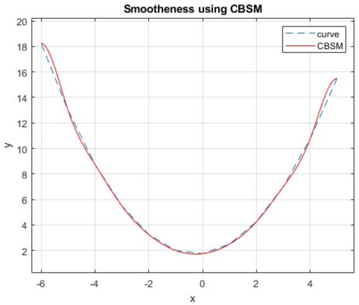

Close

Fig. 1

Smoothness from CBSM shows the end control points.

Export to PPT

When given boundary conditions in the collocation technique, the basis functions should disappear at the curve's boundary. However, in the case of cubic B-splines the basis functions $B_{-1},B_0,B_1,...,B_{N-1},B_N,B_{N+1}$ are not disappearing on one of the boundary locations (Mittal & Jain, 2012). Consequently, the basis functions need to be adjusted to form a new set that vanishes on the boundaries when the boundary conditions are applied. In order to solve this limitation, the modified term is introduced into equation (3) using a free parameter $\gamma$ , given by the equation below:

Notice that if $\gamma =-4$ , the modifying basis scheme becomes zero at the boundary point (Ito, 1975):

$v_i$ represents the constant coefficients that need to be computed and ${\overline{B}}_i\left(x\right)$ are the modified basis cubic B-splines using free parameter $\gamma =1$ .

Equation (12) is subsequently used to provide an approximation solution for ODEs by employing a diagonally dominant system. This linear equation system is obtained to control the solution of ODEs while considering the initial and boundary conditions.

The system is solved using the known Thomas method.

3 Implementation of modified basis method

In this section, the generalized process for the solution of ODEs is derived.

For this purpose, let's examine the second-order linear BVP expressed in the following form:

Solving equation (13) by using equation (12), will give equation (14) below,

4 Numerical results

In this section, the performance of MCBSM on boundary value problems of the second order ODEs is examined, and the comparisons are made with exact solutions and other existing methods. The test problems considered here are second order linear nonhomogeneous, constant coefficients BVPs. The testing is based on the different number of $N$ values for MCBSM for the second order ODEs. The maximum error $L_{\infty }$ norm is used to calculate the accuracy, which can be determined from the following formula,

Problem 1 (Latif et al., 2021): $$y^{″}-y=2\exp \left(x-1\right),y\left(0\right)=0,y\left(1\right)=1$$ With exact solution $$y=\left(x\right)\exp \left(x-1\right).$$

Problem 2 (Latif et al., 2021): $$y^{″}-y^{\prime }=-\exp \left(x-1\right)-1,y\left(0\right)=0,y\left(1\right)=0$$ With exact solution $y=(x).(1-\mathrm{e}\mathrm{x}\mathrm{p}(x-1))$ .

Problem 3 (Latif et al., 2021): $$y^{″}+y^{\prime }-6y=x,y\left(0\right)=0,y\left(1\right)=1$$ With exact solution as: $$y=\frac{\left(43-{\mathrm{e}}^2\right){\mathrm{e}}^{-3x}-(43-{\mathrm{e}}^{-3}){\mathrm{e}}^{2x}}{36({\mathrm{e}}^{-3}-{\mathrm{e}}^{-2})}-\frac{x}{6}-\frac{1}{36}$$

Problem 4 (Latif et al., 2021): $$y^{″}+2y^{\prime }+5y=6\cos \left(2x\right)-7\sin \left(2x\right),y\left(0\right)=4,y\left(\frac{\pi }{4}\right)=1$$ With exact solution as: $$y=2\left(1+e^{-x}\right)\cos \left(2x\right)+\mathrm{s}\mathrm{i}\mathrm{n}(2x)$$

Problem 5 (Basbuk et al., 2016):

Application to the Mass-spring Vibration.

Consider a free undamped motion, $y^{″}+3y=0,y\left(0\right)=0,y\left(1\right)=2$ .

With exact solution as: $$y=\frac{2\sin \left(\sqrt{3}t\right)}{\sin \left(\sqrt{3}\right)}$$ According to the absolute errors, the solution values are found to be closely related to the exact solution with the help of MATLAB. In Table 2, the proposed method is applied to problems (1 – 4) and results are compared with different values of $N=10,100$ and with the New Cubic B-spline Approximation (NCBSA) (Latif et al., 2021), Cu-B-Spline Interpolation Method (CBSIM) (Shafie & Majid, 2012; Ware and Ashine, 2021) and trigonometric Cu-B-spline (TCBSM) (Abd Hamid et al., 2010) in terms of error norms and the norms value. The generated values by the proposed method show the more closeness to the exact values. The method is applied to problem 2, and its results are compared with those of NCBSA and CBSIM at $N=10,100,1000$ in terms of error norms. The norm values generated by proposed method at $N=10$ , show the closeness to the exact value in comparison to norms values generated for $N=100$ , and $N=1000$ . For problems 3 and 4, the proposed method is then compared with NCBSA in terms of error norms at N=100 only. The norm values, given in Table 2 show better approximation data produced by the proposed method and are closer to actual solution data. Figs. 2-5 show comparisons of numerical and exact solutions to the problems (1–4). Fig. 6 shows the plotting of MCBSM when solving the problem of mass-spring vibration applications that are commonly used in many physical systems related to engineering. Notice that the MCBSM provides good convergence in comparison to the exact solutions. In conclusion, the MCBSM outperforms the competing methods which are the NCBSA (Latif et al., 2021), CBSI (Shafie & Majid, 2012; Ware and Ashine, 2021) and TCBSM (Abd Hamid et al., 2010) in terms of error norms.

Close

Fig. 2

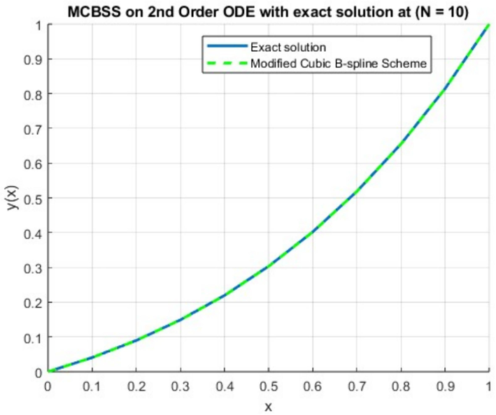
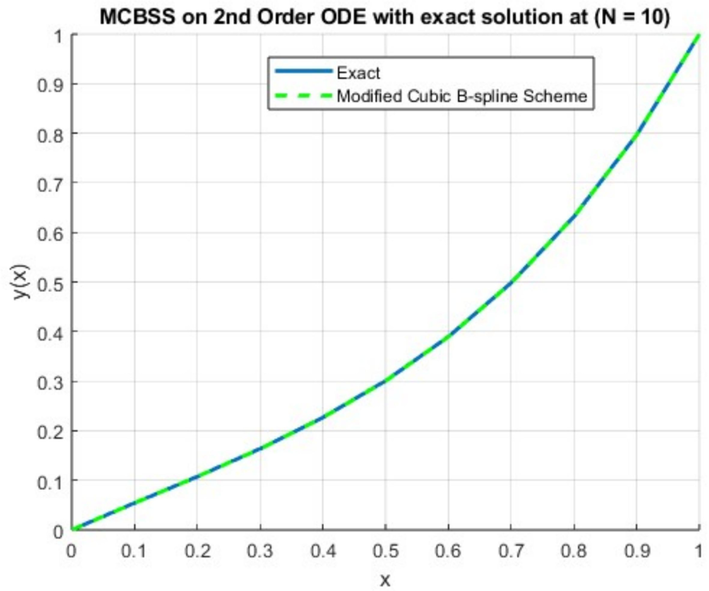
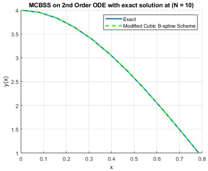
Comparison of exact and numerical solutions at N=10 for problem 1.

Export to PPT

Close

Fig. 3

Comparison of exact and numerical solutions at N=10 for problem 2.

Export to PPT

Close

Fig. 4

Comparison of exact and numerical solutions at N=10 for problem 3.

Export to PPT

Close

Fig. 5

Comparison of exact and numerical solutions at N=10 for problem 4.

Export to PPT

Close

Fig. 6

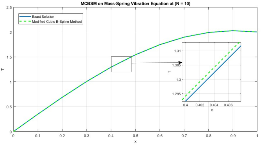
Approximate displacement of mass at different time steps N=10 with error norm 2.76463E-09.

Export to PPT

5 Discussions

In NCBSA (Latif et al., 2021) the author attempted to approximate the second derivative and find a truncation error using Taylor series expansion at cubic B-spline basis knots. However, this method faced challenges, particularly when dealing with boundary conditions, as it did not provide satisfactory results in terms of shape preservation and smoothness of the curve solution. Similarly to TCBSM (Abd Hamid et al., 2010), it only applied trigonometric basis functions to problems involving trigonometric function curves. On the other hand, CBSI (Shafie & Majid, 2012; Ware and Ashine, 2021) focused solely on interpolating given data points, excluding end control points from consideration. These methods had their own limitations, which restricted their applicability in scenarios requiring comprehensive control over the shape and behavior of the resulting curves. In contrast, the MCBSM stands out by offering substantial advantages. It excels in terms of shape preservation, ensuring smoothness in the generated curves, and reducing approximation errors when compared to traditional cubic B-splines. The key to these benefits lies in MCBSM's implementation, which employs a modified basis scheme that includes a free parameter. This parameter allows for fine-tuning the influence of control points, resulting in improved control over the shape of the curve. While other higher-order methods, including traditional cubic B-splines, suffer from issues like shape distortion and computationally intensive calculations, MCBSM addresses these concerns effectively. A comparison of smoothness and shape preservation is given in Figs. 2-6. As a result, MCBSM becomes a preferred choice in applications where precise, visually pleasing curve generation is essential and preservation of the original shape is a priority.

6 Conclusion

This study presents the numerical solution of linear two-point BVPs. The proposed method consists of a modification of the CBS basis function using a linear combination formula with a free parameter $\gamma$ together with a collocation method. MCBSM has demonstrated several favorable characteristics. Referring to Table 2, the MCBSM shows excellent approximations in terms of the second derivative as shown by the error norm when compared with other variations of CBS methods. MCBSM also allows for flexible knot placement, as shown in equations (8) and (12), which allows the authors to focus on computational efforts in the areas of interest while minimizing the computational costs.

From the convergence test computed in Section 3, the MCBSM is a second-order convergent, indicating better accuracy in approximations. It performs well for second-order BVPs and has the lowest absolute error. The accuracy of the proposed method is verified by applying it to five test problems and comparison is made corresponding to exact solutions. The numerical results of the first four test problems show that the MCBSM gives more precise and better results when compared to NCBSM, TCBSM, and CBSI in terms of error norms. It is worth to highlight that, in general, the errors decreased as the $N$ increased with a decreased in the step size, and the method achieved higher accuracy. Hence, it can be concluded that the MCBSM is effective in solving linear two-point BVPs.

Funding

The first author is supported by Graduate Assistantship Scheme (GA) to pursue his Ph.D. study at Universiti Teknologi PETRONAS (UTP) and the paper is funded by a YUTP Grant under the cost centre: 015LC0-315, Universiti Teknologi PETRONAS, Malaysia.

CRediT authorship contribution statement

Mudassar Iqbal: Writing – original draft, Visualization, Software, Methodology, Formal analysis, Conceptualization. Nooraini Zainuddin: Writing – original draft, Validation, Supervision, Software, Methodology, Formal analysis. Hanita Daud: Validation, Supervision. Ramani Kanan: Writing – original draft, Validation, Supervision, Funding acquisition. Hira Soomro: Writing – review & editing, Formal analysis. Rahimah Jusoh: Validation. Atta Ullah: Formal analysis. Iliyas Karim Khan: Formal analysis.

References

- New cubic b-spline approximations for solving non-linear third-order korteweg-de vries equation. Indian J. Sci. Technol. 2019;12(15):1-9.
- [Google Scholar]
- Cubic trigonometric B-spline applied to linear two-point boundary value problems of order two. Int. J. Math. Comput. Sci.. 2010;4(10):1377-1382.
- Extended cubic B-spline method for linear two-point boundary value problems. Sains Malaysiana. 2011;40(11):1285-1290.
- Boundary Value Problems from Higher Order Differential. Equations: World Scientific; 1986.
- Vibration analysis of a mass on a spring by means of magnus expansion method. New Trends Math. Sci.. 2016;4(2):90.
- [CrossRef] [Google Scholar]
- B-spline interpolation compared with finite difference, finite element and finite volume methods which applied to two-point boundary value problems. Appl. Math Comput.. 2006;175(1):72-79.
- B-spline method for solving linear system of second-order boundary value problems. Comput. Math. Appl.. 2009;57(5):757-762.
- Finite difference, finite element and finite volume methods applied to two-point boundary value problems. J. Comput. Appl. Math.. 2002;139(1):9-19.
- Construction and application of nine-tic B-spline tensor product SS. Mathematics. 2019;7(8):675.
- Extended cubic B-spline method for solving a system of non-linear second-order boundary value problems. J. Math. Comput. Sci. 2020;21:231-242.
- Hybrid cubic b-spline method for solving Non-linear two-point boundary value problems. Int. J. Pure Appl. Math. 2016;110(2):369-381.
- A numerical approach for an epidemic SIR model via Morgan-Voyce series. Int. J. Math. Comput. Eng.. 2024;2(1):125-140.
- New cubic B-spline approximation for solving third order Emden-Flower type equations. Appl. Math Comput.. 2018;331:319-333.
- Convexity Preservation of the Ternary 6-point Interpolating Subdivision Scheme Towards Intelligent Systems Modeling and Simulation. In: With Applications to Energy, Epidemiology and Risk Assessment. Springer; 2021. p. :1-23.
- Construction and application of Septic B-spline tensor product scheme. Advanced Methods for Processing and Visualizing the Renewable Energy: A New Perspective from Signal to Image Recognition. 2021;101–120
- Numerical solution of heat equation using modified cubic B-spline collocation method. J. Adv. Res. Numer. Heat Transfer. 2024;20(1):23-35.
- A collocation method for two-point boundary value problems. Math. Comput.. 1975;29(131):761-776.
- Solving coupled non-linear higher order BVPs using improved shooting method. Int. J. Math. Comput. Eng. 2024
- Solutions of BVPs arising in hydrodynamic and magnetohydro-dynamic stability theory using polynomial and non-polynomial splines. Alex. Eng. J.. 2021;60(1):941-953.
- Soliton propagation under diffusive and nonlinear effects in physical systems; (1+1)–dimensional MNW integrable equation. Phys. Lett. A. 2023;480
- A novel perspective for simulations of the modified equal-width wave equation by cubic Hermite B-spline collocation method. Wave Motion. 2024;129
- New cubic B-spline approximation for solving linear two-point boundary-value problems. Mathematics. 2021;9(11):1250.
- Numerical solution of the coupled viscous Burgers’ equation. Commun. Nonlinear Sci. Numer. Simul.. 2011;16(3):1304-1313.
- Numerical solutions of nonlinear Burgers’ equation with modified cubic B-splines collocation method. Appl. Math Comput.. 2012;218(15):7839-7855.
- A novel approach for Benjamin-Bona-Mahony equation via ultraspherical wavelets collocation method. Int. J. Math. Comput. Eng. 2024
- Solving the generalized equal width wave equation via sextic B-spline collocation technique. Int. J. Math. Comput. Eng.. 2023;1(2):229-242.
- A new quintic B-spline approximation for numerical treatment of Boussinesq equation. J. Math. Comput. Sci. 2020;20(1):30-42.
- A novel perspective for simulations of the MEW equation by trigonometric cubic B-spline collocation method based on Rubin-Graves type linearization. Comput. Meth. Different. Eq.. 2022;10(4):1046-1058.
- Sabir, Z., Raja, M. A. Z., Shoaib, M., Sadat, R., & Ali, M. R. J. E. w. C. (2022). A novel design of a sixth-order nonlinear modeling for solving engineering phenomena based on neuro intelligence algorithm. 1-16.
- Integration of the RLW equation using higher-order predictor–corrector scheme and quintic B-spline collocation method. Math. Sci. 2022
- Approximation of cubic B-spline interpolation method, shooting and finite difference methods for linear problems on solving linear two-point boundary value problems. World Appl. Sci. J. 2012;17:1-9.
- Trigonometric B-spline based ε-uniform scheme for singularly perturbed problems with Robin boundary conditions. J. Differ. Equations Appl.. 2022;28(7):924-945.
- A new scheme using cubic B-spline to solve non-linear differential equations arising in visco-elastic flows and hydrodynamic stability problems. Mathematics. 2019;7(11):1078.
- Sensitivity analysis-based control strategies of a mathematical model for reducing marijuana smoking. AIMS Bioengineering. 2023;10(4):491-510.
- Sensitivity analysis-based validation of the modified NERA model for improved performance. J. Adv. Res. Appl. Sci. Eng. Technol.. 2023;32(3):1-11.
- Mathematical model with sensitivity analysis and control strategies for marijuana consumption. Partial Different. Eq. Appl. Math.. 2024;10:100657
- A variational approach to nonlinear two-point boundary value problems. Comput. Math. Appl.. 2009;58(11–12):2452-2455.
- Cubic spline and finite difference method for solving boundary value problems of ordinary differential equations. Asian J. Adv. Res.. 2021;9(4):1-43.
- A new extended B-spline approximation technique for second order singular boundary value problems arising in physiology. J. Math. Comput. Sci. 2019;19(4):258-267.
- Yağmurlu, N. M., & Karakaş, A. S. (2020). Numerical solutions of the equal width equation by trigonometric cubic B-spline collocation method based on Rubin–Graves type linearization. 36(5), 1170-1183. doi:https://doi.org/10.1002/num.22470.
- Cubic spline solutions of the ninth order linear and non-linear boundary value problems. Alex. Eng. J.. 2022;61(12):11635-11649.