A Liu-Storey-type conjugate gradient method for unconstrained minimization problem with application in motion control

1 Introduction

In this paper, we present alternative nonlinear conjugate gradient (CG) method for solving unconstrained optimization problems.

Conjugate gradient methods are preferable among other optimization methods because of low storage requirements (Hager and Zhang, 2006). Based on these, a considerable amount of research articles have been published, most of these articles considered global convergence of the conjugate gradient methods that are previously difficult to globalize (see, for example, Zhang et al., 2006; Gilbert and Nocedal, 1992; Al-Baali, 1985; Dai et al., 2000). In other perspective, some articles considered widening the applicability as well as improving the numerical performance of the existing conjugate gradient methods (see for example Yuan et al., 2019; Yuan et al., 2020; Hager and Zhang, 2013; Ding et al., 2010; Xie et al., 2009; Xie et al., 2010; Abubakar et al., 2021; Abubakar et al., 2021; Malik et al., 2021).

Consider the unconstrained optimization problem

The parameter ${\alpha }_k>0$ is the steplength obtained by either the standard Wolfe line search conditions (Sun and Yuan, 2006), namely,

The scalar ${\beta }_k$ is known as the conjugate gradient parameter. Some notable parameters are; the Hestenes-Stiefel (HS) (Hestenes and Stiefel, 1952), Polak-Ribiére-Polyak (PRP) (Polak and Ribiere, 1969; Polyak, 1969) and Liu-Storey (LS) (Liu and Storey, 1991). They are defined as follows: $${\beta }_k^{\mathit{HS}}=\frac{g_k^T{y}_{k-1}}{d_{k-1}^T{y}_{k-1}}{\beta }_k^{\mathit{PRP}}=\frac{g_k^T{y}_{k-1}}{\Vert g_{k-1}{\Vert }^2},{\beta }_k^{\mathit{LS}}=\frac{g_k^T{y}_{k-1}}{-g_{k-1}^T{d}_{k-1}}\text{.}$$ where $g_k=g\left(x_k\right),y_{k-1}=g_k-g_{k-1}$ .

It can be observed that the HS, PRP, and LS method have similarity in their numerator, this similarity makes them have some common features in terms of computational performance. There exists many works on the development of the HS and PRP methods (see, for example, Zhang et al., 2007; Dong et al., 2017; Yu et al., 2008; Saman and Ghanbari, 2014; Andrei, 2011; Yuan et al., 2021), however, as noticed by Hager and Zhang (2006) in their review article, the research on the LS method is rare. Nevertheless, some works on the LS parameter have been presented in the references (Shi and Shen, 2007; Tang et al., 2007; Zhang, 2009; Liu and Feng, 2011; Li and Feng, 2011. In Shi and Shen, 2007; Tang et al., 2007; Liu and Feng, 2011), the authors proposed a new form of Armijo-like line search strategy and used it to investigate the global convergence of the LS method. Zhang (2009), developed a new descent LS-type method based on the memoryless BFGS update and proved the global convergence of the method for general function using the Grippo and Lucidi (1997) line search. Li and Feng (2011), remarked that because of the similarity of the HS, PRP, and LS conjugate parameters, the techniques applied to the HS and PRP can be applied to the LS method to improve its convergence and computational performance. In this regard, Li and Feng, proposed a modification of the LS method similar to the well-known Hager and Zhang CG-DESCENT (Hager and Zhang, 2005).

Noticing the above development, in this paper, we seek another alternative LS-type method following the modifications of the HS and PRP methods by Liang et al. (2015) and Aminifard and Saman (2019), respectively. Motivated by the above proposals and the similarity of the LS CG parameter with HS and PRP parameters, we present an efficient descent LS-type method for nonconvex functions. The direction satisfy the sufficient descent property without any line search requirement and the method is globally convergent under the standard Wolfe line search as well as the Armijo-like line search. The rest of the paper is organized as follows. In Section 2 we provide the algorithm of the descent LS -type method together with its convergence result. In Section 3, we present the numerical experiments, and conclusions are given in Section 4. Unless otherwise stated, throughout this paper we denote $g_k=g(x_k)$ .

2 Algorithm and theoretical results

Recently, some proposals have been made to modify the HS and PRP methods. The proposal to modify the HS method was done by Liang et al. (2015) and that to modify the PRP (named as NMPRP method) was done by Aminifard and Saman (2019). In Liang et al. (2015), some CG methods with a descent direction was presented. Moreover, the conjugacy condition given by Dai and Liao (2001) was extended. Likewise in Aminifard and Saman (2019), a descent extension of the PRP method was presented and the global convergence was shown under the Wolfe and Armijo-like line search, respectively. In this section, we build on the analysis given in Liang et al. (2015) and Aminifard and Saman (2019) on the LS method to guarantee a sufficient descent direction (3).

Note that if ${\beta }_k^{\mathit{LS}}⩾0$ , then condition (3) is satisfied when $g_k^T{d}_{k-1}⩽0$ . Now, our interest is to consider the case where $g_k^T{d}_{k-1}>0$ and the direction satisfies (3). To achieve this, we attach a scaling parameter ${\gamma }_k$ to the term $-g_k$ in (2) and propose the following search direction

It is worth noting that if the exact line search is used, the parameter ${\beta }_k^{\mathit{MLS}}$ reduces to ${\beta }_k^{\mathit{LS}}$ . If $g_k^T{y}_{k-1}⩽0$ the direction $d_k^{\prime }$ defined in (7) may not necessarily be descent, in this case we set $d_k^{\prime }=-g_k$ . Therefore, we defined the proposed direction by

It can be observed that a restart process for the CG method with direction $d_k^{\prime }$ defined by (7) occur when $g_k^T{y}_{k-1}⩽0$ .

Below we give the algorithm flow framework of the proposed scheme.

Algorithm 1: New Modified LS method (NMLS)

Next, we prove the convergence of Algorithm 1 under the standard Wolfe line search conditions (4)-(5). In addition, we employ the following assumptions.

Assumptions 2.3 and 2.4 implies that for all $x\in \mathcal{H}$ there exists $c_1,c_2>0$ such that;

• $\Vert x\Vert ⩽c_1$ .

• $\Vert g(x)\Vert ⩽c_2$ .

• $\{x_k\}\in \mathcal{H}$ as $\{f(x_k)\}$ is decreasing.

In what follows, we prove the convergence result of Algorithm 1 under the Armijo-like condition (6).

Since $\{f(x_k)\}$ is nonincreasing, using (6) we have $${\displaystyle \sum _{k=0}^{\infty }}{\alpha }_k^2\Vert d_k{\Vert }^2<+\infty ,$$ which further implies that

3 Numerical examples

This section demonstrates the numerical performance of Algorithm 1. Algorithm 1 is named as NMLS method. Based on the number of iteration (NOI), the number of function evaluations (NOF), and central processing unit (CPU) time, we compare the performance of the NMLS method with the NMPRP method (Aminifard and Saman, 2019). Fifty-six (56) test functions suggested by Andrei (2017) and Jamil (2013) are selected for testing the computational performance of each method. For each test function, we run two problems with different starting points or variation dimensions of 2, 4, 8, 10, 50, 100, 500, 1000, 5000, 10000, 50000 and 100000. The list of test functions is given in Table 1. The algorithm was coded in MATLAB R2019a and compiled on a PC with specification: processor Intel Core i7, operating system Windows 10 pro 64 bit, and 16 GB RAM. We stop the algorithm when $\Vert g_k\Vert ⩽{10}^{-6}$ , and the numerical results are said to fail (use “–” to report the failure), if one of the conditions is satisfied: the NOI is more than 10,000 or the problem fail to attained the optimum value.

In this section, we compare the proposed NMLS method with NMPRP method using the strong Wolfe and Armijo-like line searches. This is done as a fair comparison adapted to the NMPRP method in Aminifard and Saman (2019). We use the strong Wolfe conditions comprises of (4) and the following stronger version of (5): $$|g_{k+1}^T{d}_k|⩽-\sigma g_k^T{d}_k\text{.}$$

To obtain the step-size ${\alpha }_k$ by using strong Wolfe line search in the NMLS method, the parameters are selected as $\sigma =0.05$ and $\vartheta =0.0001$ . Meanwhile, under the Armijo-like line search, we use the parameters $\rho =0.25$ and $\delta =0.00003$ . For good performance, we choose the parameter $t=0.1$ for evaluating ${\beta }_k^{\mathit{MLS}}$ . In the NMPRP method, we still maintain all the parameter values according to the article (Aminifard and Saman, 2019). All numerical results under the strong Wolfe line search are shown in Table 2 and under Armijo-like line search are given in Table 3. The items in each table have the following meanings: Funct.: the test function, Dim.: dimension, and IP: arbitrary initial points. From the numerical results in Tables 2 and 3, we can see that the NMLS method in this paper is promising.

On the other hand, we use the performance profile introduced by Dolan and Moré (2002) to compare and evaluate the performance of NMLS and the NMPRP methods. The performance profile of each method is depicted by a segment of each problem to obtain a profile curve. From the profile curve, the method that top the curve has the best performance.

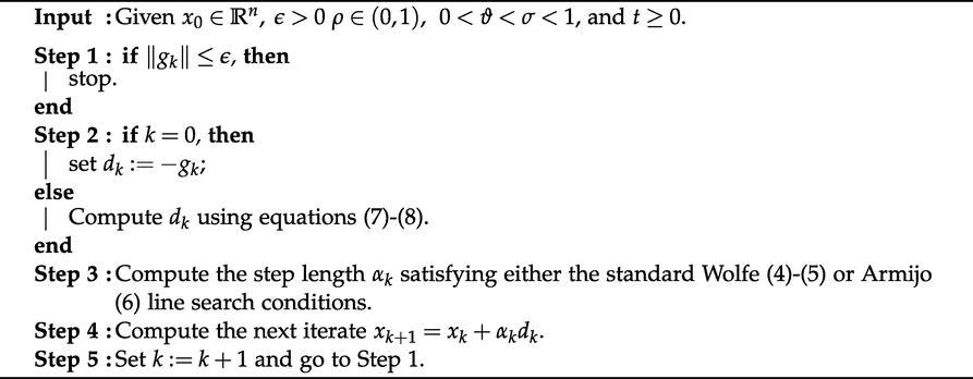
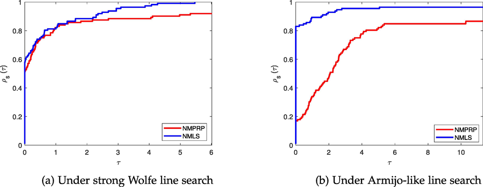
Figs. 1–3 present the performance profile with respect to the three metrics; NOI, NOF and CPU time of the two methods, respectively. From Fig. 1a, Fig. 1b, Fig. 2a, Fig. 2b, Fig. 3a, and Fig. 3b, the proposed NMLS method has the best performance based on all metrics under strong Wolfe line search and Armijo-like line search.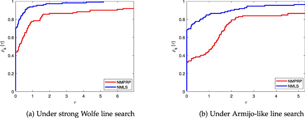

Close

Fig. 1

Performance profile based on NOI.

Export to PPT

Close

Fig. 2

Performance profile based on NOF.

Export to PPT

Close

Fig. 3

Performance profile based on CPU time.

Export to PPT

3.1

3.1 Application in motion control

This subsection test the efficiency of Algorithm 1 in solving motion control problem. Algorithm 1 (NMLS method) is implemented using the Armijo-like line search (6), in which we set $\rho =0.6,t={10}^{-14}$ and $\vartheta =0.018$ . We begin with a brief background on motion control problems (Zhang et al., 2019; Sun et al., 2020). Here we look only at the motion control of two-joint planar robot manipulator. Given the path of the vector desired $r_{\mathit{dk}}\in {\mathcal{R}}^2$ at time instant $t_k\in [0,t_f]$ , the discrete-time kinematics equation is: finding ${\theta }_k\in {\mathcal{R}}^2$ such that $$f({\theta }_k)=r_{\mathit{dk}}\text{.}$$

f is a mapping given by $$f(\theta )=\left[\begin{array}{c}{l}_1{c}_1+l_2{c}_2\hfill \\ l_1{s}_1+l_2{s}_2\hfill \end{array}\right],$$ where $c_1=\cos ({\theta }_1),s_1=\sin ({\theta }_1),c_2=\cos ({\theta }_1+{\theta }_2),s_2=\sin ({\theta }_1+{\theta }_2)$ , and $l_i$ denote the i-th rod length. Obviously, this problem can be described as a minimization problem

(21)

$${\displaystyle \underset{{\theta }_k\in {\mathcal{R}}^2}{\min }}\frac{1}{2}\Vert f({\theta }_k)-r_{\mathit{dk}}{\Vert }^2\text{.}$$

For simplicity, we set $l_i=1(i=1,2)$ and the end-effector is controlled to track the following Lissajous curve (Zhang et al., 2019) $$r_{\mathit{dk}}=\left[\begin{array}{c}1.5+0.2\sin (\pi t_k/5)\hfill \\ \sqrt{3}/2+0.2\sin (2\pi t_k/5+\pi /3)\hfill \end{array}\right]\text{.}$$

The starting point of the initial problem is ${\theta }_0={[0,\pi /3]}^{\top }$ , and that of any i-th problem is the approximate solution to the $i-1$ -th problem ( $i=2,3,\cdots$ ). Furthermore the time for the task is $[0,10]$ , and divided equally into 200 pieces. The outcomes obtained by NMLS are presented in Fig. 4, which shows that NMLS algorithm effectively accomplished the task. More specifically, synthesization of the trajectories of the robot using the NMLS algorithm is plotted in Fig. 4a, and trajectory of end-effector as well as the path desired are plotted in Fig. 4b. Figs. 4c and 4d show the error generated by the NMLS method on x-axis and y-axis, respectively. It is not easy to see the variation of the generated end-effector trajectory and desired path from Fig. 4a and 4b. Actually, Fig. 4c and 4d depict that the errors are not above ${10}^{-5}$ . 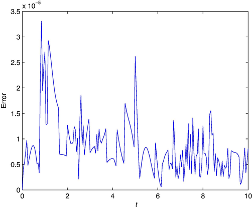In addition, to show the absolute error generated by NMLS, we show their Euclidean distance of end-effector trajectory and desired path in Fig. 5, from which we find that the absolute error is always smaller than $3.5\times {10}^{-5}$ . This shows that NMLS completes the task with high precision. In Fig. 4a there is one broken line that is far from other broken lines, which indicates that there is some sudden shift of the manipulator. This may cause damage to the manipulator. Therefore, in addition to the unconstrained optimization model (21), we need to design some new mathematical model of this motion control, which can generate continuous and repetitive motion control. This is one of our further research topics.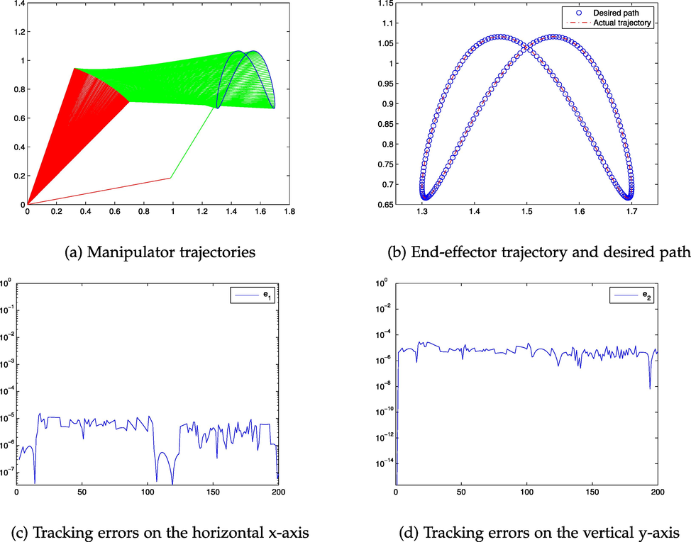

Close

Fig. 4

Numerical results generated by NMLS.

Export to PPT

Close

Fig. 5

Absolute error generated by NMLS.

Export to PPT

4 Conclusions

In this article, we have presented a Liu-Storey type conjugate gradient method that guarantees sufficient descent condition independent of the line search. Using the Wolfe and Armijo-like line search conditions, we proved that the NMLS method converges globally. Moreover, the presented method can inherit a built-in self-restarting mechanism of the LS method. Based on our numerical findings, we conclude that the proposed method is the most efficient and promising.

References

- A hybrid FR-DY conjugate gradient algorithm for unconstrained optimization with application in portfolio selection. AIMS Math.. 2021;6(6):6506-6527.
- [Google Scholar]
- A hybrid conjugate gradient based approach for solving unconstrained optimization and motion control problems. Math. Comput. Simul. 2021
- Descent property and global convergence of the Fletcher-Reeves method with inexact line search. IMA J. Numer. Anal.. 1985;5(1):121-124.
- A modified descent Polak–Ribiére–Polyak conjugate gradient method with global convergence property for nonconvex functions. Calcolo. 2019;56(2):16.
- Andrei, N., 2011. A modified Polak–Ribière–Polyak conjugate gradient algorithm for unconstrained optimization. Optimization 60(12), 1457–1471.
- Accelerated adaptive perry conjugate gradient algorithms based on the self-scaling memoryless bfgs update. J. Comput. Appl. Math.. 2017;325:149-164.
- New conjugacy conditions and related nonlinear conjugate gradient methods. Appl. Math. Optim.. 2001;43(1):87-101.
- Convergence properties of nonlinear conjugate gradient methods. SIAM J. Optim.. 2000;10(2):345-358.
- Iterative solutions to matrix equations of the form aixbi=fi. Comput. Math. Appl.. 2010;59(11):3500-3507.
- Benchmarking optimization software with performance profiles. Math. Program.. 2002;91(2):201-213.
- Some new three-term Hestenes-Stiefel conjugate gradient methods with affine combination. Optimization. 2017;66(5):759-776.
- Global convergence properties of conjugate gradient methods for optimization. SIAM J. Optim.. 1992;2(1):21-42.
- globally convergent version of the polak-ribière conjugate gradient method. Math. Program.. 1997;78(3):375-391.
- A new conjugate gradient method with guaranteed descent and an efficient line search. SIAM J. Optim.. 2005;16(1):170-192.
- survey of nonlinear conjugate gradient methods. Pacific J. Optim.. 2006;2(1):35-58.
- The limited memory conjugate gradient method. SIAM J. Optim.. 2013;23(4):2150-2168.
- Methods of conjugate gradients for solving linear systems. J. Res. Natl. Bureau Standards. 1952;49(6):409-436.
- A literature survey of benchmark functions for global optimisation problems. Int. J. Math. Model. Numer. Optim.. 2013;4(2):150-194.
- A sufficient descent LS conjugate gradient method for unconstrained optimization problems. Appl. Math. Comput.. 2011;218(5):1577-1586.
- A modified Hestenes-Stiefel conjugate gradient method with sufficient descent condition and conjugacy condition. J. Comput. Appl. Math.. 2015;281:239-249.
- Global convergence of a modified LS nonlinear conjugate gradient method. Proc. Eng.. 2011;15:4357-4361.
- Efficient generalized conjugate gradient algorithms, part 1: theory. J. Optim. Theory Appl.. 1991;69(1):129-137.
- Malik, M., Abubakar, A.B., Sulaiman, I.M., Mamat, M., Abas, S.S., Sukono. 2021. A new three-term conjugate gradient method for unconstrained optimization with applications in portfolio selection and robotic motion control. Int. J. Appl. Math. 51(3).
- Note sur la convergence de méthodes de directions conjuguées.Revue française d’informatique et de recherche opérationnelle. Vol 3. Série rouge; 1969. p. :35-43.
- The conjugate gradient method in extremal problems. USSR Computational Mathematics and Mathematical Physics. 1969;9(4):94-112.
- Saman, B.-K., Ghanbari, R., 2014. A descent extension of the Polak–Ribière–Polyak conjugate gradient method. Comput. Math. Appl. 68(12), 2005–2011.
- Convergence of Liu-Storey conjugate gradient method. Eur. J. Oper. Res.. 2007;182(2):552-560.
- Sun, W., Yuan, Y. Optimization theory and methods: Nonlinear programming. Springer (992).
- Two improved conjugate gradient methods with application in compressive sensing and motion control. Math. Problems Eng.. 2020;2020
- G.A new version of the Liu-Storey conjugate gradient method. Appl. Math. Comput.. 2007;189(1):302-313.
- Gradient based iterative solutions for general linear matrix equations. Comput. Math. Appl.. 2009;58(7):1441-1448.
- Gradient based and least squares based iterative algorithms for matrix equations axb+cxtd=f. Appl. Math. Comput.. 2010;217(5):2191-2199.
- The global convergence of the Polak–Ribière–Polyak conjugate gradient algorithm under inexact line search for nonconvex functions. J. Comput. Appl. Math.. 2019;362:262-275.
- The PRP conjugate gradient algorithm with a modified wwp line search and its application in the image restoration problems. Appl. Numer. Math.. 2020;152:1-11.
- The modified PRP conjugate gradient algorithm under a non-descent line search and its application in the muskingum model and image restoration problems. Soft. Comput.. 2021;25(8):5867-5879.
- Global convergence of modified Polak-Ribière-Polyak conjugate gradient methods with sufficient descent property. J. Ind. Manage. Optim.. 2008;4(3):565.
- Zhang L., 2009. A new Liu–Storey type nonlinear conjugate gradient method for unconstrained optimization problems. J. Comput. Appl. Math. 225(1), 146–157.
- A descent modified Polak–Ribière–Polyak conjugate gradient method and its global convergence. IMA J. Numer. Anal.. 2006;26(4):629-640.
- Some descent three-term conjugate gradient methods and their global convergence. Optim. Methods Software. 2007;22(4):697-711.
- General four-step discrete-time zeroing and derivative dynamics applied to time-varying nonlinear optimization. J. Comput. Appl. Math.. 2019;347:314-329.
Appendix A
See Tables 2 and 3.
Func.
Dim.
IP
NMPRP
NMLS
NOI
NOF
CPU Time
F1
50000
(1.1,…,1.1)
27
114
2.1063
10
59
0.9867
100000
3.8852
58
1.9118
F2
(0.1,1,…,0.1,1)
133
0.9388
16
75
0.5461
1.8728
1.0683
F3
(0.5,−2,…,0.5,−2)
–
8
38
0.2869
0.5809
F4
(1,0.8,…,1,0.8)
56
1.0577
44
0.8081
2.1137
1.6154
F5
50
(2,…, 2)
66
177
0.0066
82
991
0.0254
100
(2,…,2)
71
216
0.0125
220
1837
0.1142
F6
(−2.1,…,−2.1)
83
217
4.164
48
0.7848
97
303
11.2897
47
1.5565
F7
(0.1,…,0.1)
9
24
0.1955
21
0.1716
0.3747
0.3468
F8
(5,…,5)
40
0.3006
13
103
0.678
0.5847
11
0.7318
F9
(−5,…,−5)
39
175
1.222
363
2.3116
37
159
2.2551
55
246
3.3653
F10
(8,…,8)
160
607
11.0454
195
799
14.369
245
1103
38.2768
84
421
14.5381
F11
(1.05,…,1.05)
26
81
0.629
41
125
0.9895
30
1.5444
249
3.3063
F12
(1,…,1)
7
22
0.1765
6
20
0.1677
0.3481
0.3149
F13
500
(−10,…,−10)
120
0.0167
152
0.0344
1000
329
0.0638
284
0.0629
F14
(1.05, …, 1.05)
19
0.0018
116
0.0053
25
76
0.0083
347
0.0165
F15
104
0.003
68
0.0039
15
91
0.0095
F16
2
(−1.5,−2)
4.40E−03
28
4.05E−04
(−5,−10)
70
0.0014
45
4.88E−04
F17
(−5,−5)
18
6.09E−04
507
0.0041
(5,5)
0.0011
0.0026
F18
3.70E−03
2.86E−04
(10,10)
1.50E−04
1.49E−04
F19
(−1,0.5)
1
3
9.78E−05
7.70E−05
(−5,5)
36
5.95E−04
74
4.41E−04
F20
(0,0)
7.80E−03
1.19E−04
0.0017
14
67
8.19E−04
F21
(1.001,…,1.001)
0.3292
5
0.1546
0.6534
0.2997
F22
141
0.8757
169
1.9728
F23
176
0.0112
200
2568
0.0903
190
582
0.1224
328
2856
0.4666
F24
(−2.5,−2.5)
34
198
0.0016
163
(−8.5,−8.5)
53
429
0.0048
412
0.0034
F25
29
112
0.0033
146
0.0038
155
0.0155
F26
79
532
0.0127
604
0.0388
F27
(3,…,3)
143
0.0215
438
0.0284
1574
4722
0.9696
1584
4753
0.9698
F28
187
561
0.1345
209
872
0.175
10000
606
1818
3.6627
695
2792
5.0326
F29
179
0.0106
298
0.0193
42
401
0.0713
510
0.086
F30
(2.5,…,2.5)
0.0019
0.0023
72
0.0075
61
0.0065
F31
4
(10,10,10,10)
222
0.0036
1581
9824
0.0624
(100,…,100)
62
346
0.006
1102
6668
0.0515
F32
(1,1)
63
252
0.004
(20,20)
80
320
0.005
5.27E−04
F33
(1.01,…,1.01)
0.001
201
31
106
0.0032
542
0.0027
F34
271
158
1743
0.0185
224
969
0.0445
1494
16304
0.4986
F35
0.0305
0.0345
0.0534
F36
5000
(−1,…,−1)
435
1305
1.1682
477
1431
1.2797
1399
4197
32.1167
1578
4778
41.4889
F37
0.1518
0.1121
1.2014
0.8156
F38
17
0.1517
0.0767
0.7345
0.5609
F39
(1.02,…,1.02)
23
0.0909
12
78
0.075
0.7157
87
0.7222
F40
0.041
0.0353
0.0684
0.064
F41
213
1.4846
1.3216
208
2.84
2.6386
F42
703
3432
0.1174
2457
0.0901
877
4989
0.9623
692
7470
1.3607
F43
85
263
0.0056
281
0.0131
F44
321
7917
0.0366
361
9535
0.0483
344
8358
0.0532
269
7078
0.0449
F45
445
1335
1.1661
479
1573
1.2648
633
1899
3.456
686
2355
4.1385
F46
(4,…,4)
847
16.2004
51
0.9805
105
879
33.5407
1.9413
F47
3071
0.1165
134
2434
0.0815
444
5685
0.6422
405
6495
0.7
F48
3610
0.0173
3715
0.0241
1044
18579
0.0832
18565
0.0705
F49
2.48E−04
2.07E−04
(8,8)
1.52E−04
F50
8.14E−04
(−1,−1)
8.72E−04
F51
(2.5,2.5)
8.75E−04
8.20E−04
170
0.0028
0.0012
F52
(4,4)
89
0.002
9.97E−04
(1.5,1.5)
0.0035
F53
5.97E−04
3.96E−04
3.39E−04
2.95E−04
F54
(0.4,…,0.4)
398
5203
0.5884
327
5272
0.5708
2276
32993
24.4614
577
9468
6.7099
F55
(1,2,…,10000)
304
0.4694
300
0.4533
(1,2,…,50000)
353
2.0584
260
1.4967
F56
0.0118
210
0.0108
35
203
0.0527
33
293
0.0549
343
8414
36.5449
1014
7.9958
334
8160
69.2095
1710
34.4755
274
6083
5.1683
121
1059
1.9011
6101
14.229
162
1282
5.7396
317
8333
8.125
285
7565
13.0259
193
2408
20.5074
640
5.3248
2420
58.852
165
1290
37.4979
88
558
0.6429
102
770
145
1217
0.0393
2210
722
1328
57.5115
863
867
31.0011
864
1718
154.1461
982
986
148.3827
2367
2.7513
776
1.3088
2282
5.3768
537
2.4787
2406
2.5317
54
385
0.8655
2456
5.1637
402
1.8747
345
8110
0.0266
530
0.0057
3015
67319
0.924
1760
0.0654
4678
0.0934
1879
24291
0.3753
373
5820
0.7372
22603
2.9481
2366
3.1738
52
0.8185
49
456
1.7689
86
635
1.2963
0.4912
570
2.5959
0.902
129
1896
0.0146
499
132
0.0242
101
778
0.018
95
685
0.009
313
128
1052
0.0307
332
0.0124
211
4583
2895
196
4341
0.0433
2503
856
1.76E−01
171
6.46E−04
839
0.0045
140
153
9.63E−04
90
783
1.10E−03
912
0.0037
1169
9.60E−02
7.35E−04
613
0.0049
335
3.60E−03
0.0171
60
431
0.0021
174
2401
458
0.9017
425
0.7686
64
483
1.779
98
915
2.824
0.3194
0.6645
2640
0.0262
1352
0.1293
9686
0.1551
5068
0.1918
248
6066
0.1254
243
2652
0.0091
5233
0.0132
275
3165
0.0062
156
2024
0.0145
0.0047
2333
0.0403
0.007
0.0074
111
721
0.0141
15491
0.0399
1088
11492
0.0476
1119
37179
0.1394
1871
22067
0.1567
351
8188
0.1416
618
5406
1.2305
1141
35261
5.9839
7386
108554
37.9789
311
10782
0.0308
3486
74335
0.3662
461
19621
0.2568
378
4864
0.1917
1572
0.0061
261
7.87E−04
2356
0.0123
2.35E−01
239
5724
0.022
393
3887
0.0329
325
8204
0.0209
371
3912
0.021
0.0055
0.0067
342
5802
0.0134
630
0.0059
267
6510
0.0136
436
0.0024
151
1872
131
1067
677
15030
0.0698
683
4526
0.0581
1847
1.0773
0.3573
2447
2.4575
0.6896
404
10324
0.1742
733
7743
0.2627
855
26517
1.4923
2773
41336
4.8455
601
1.075
147
0.2807
660
8.7063
251
3.2634
167
3485
0.3386
369
0.0935
180
3727
3.6781
380
0.7706
0.0731
168
0.5191
340
0.803
331
1.4508
2546
26486
0.14
6631
85547
1.8229
254
8876
0.0498
1519
32237
0.1569
264
8837
0.1669
1155
25694
0.6078
117
1215
257
1228
1845
443
126
1576
680
0.0031
911
28172
1.7493
3566
54740
5.7253
1319
43903
7.0819
1523
15798
6.044
2486
20.6921
0.0436
2500
39.4022
2750
0.0263
2152
0.0273
123
2900
0.0584
1711
0.0594
1035
262
0.0025
1114
0.0077
9.23E−04
1534
1873
0.0043
6.77E−04
135
2608
3088
0.0148
184
137
2918
0.0102
487
5529
0.0249
92
1244
0.0046
2570
41676
0.0856
2880
0.0063
516
238
2579
0.0506
2992
0.0759
3089
0.2593
242
2559
0.382
(1,2,…,100)
1531
0.0217
232
(1,2,…,500)
2301
0.0566
43
0.032
2736
0.031
109
1009
441
12977
0.4352
1756
0.0878
Appendix B
Supplementary data
Supplementary data associated with this article can be found, in the online version, at https://doi.org/10.1016/j.jksus.2022.101923.
The following are the Supplementary data to this article: