

Translate this page into:
A hybrid method for solving fuzzy Volterra integral equations of separable type kernels
⁎Corresponding author at:Department of Mathematics and General Sciences, Prince Sultan University, Riyadh, Saudi Arabia. tabdeljawad@psu.edu.sa (Thabet Abdeljawad),
-
Received: ,
Accepted: ,
This article was originally published by Elsevier and was migrated to Scientific Scholar after the change of Publisher.
Abstract
The paper deals with the computation of solutions of fuzzy Volterra integral equations with degenerate kernel by applying a hybrid method. The proposed method is built on Laplace transform coupled with Adomian Decomposition Method; Laplace Adomian Decomposition Method abbreviated as (LADM). In the considered equation the unknown function has a solution in terms of infinite series expansion and hence LADM becomes more accurate to give the exact solution. Firstly, using the fuzzy number in term of parametric form, the fuzzy Volterra integral equation is converted to two crisp integral equations and then LADM is applied to get the exact fuzzy solutions of fuzzy linear Volterra integral equations. For the illustration, some examples of considered equations are solved to highlight the robustness, efficiency and the applicability of the developed scheme. The obtained results play an important role in developing the theory of fuzzy analytical dynamic equations.
Keywords
Fuzzy linear Volterra integral equation
Laplace Adomian Decomposition Method (LADM)
Fuzzy number in parametric form
Degenerate kernel

1 Introduction
The study of fuzzy integral equations is of more interest and fast growing, especially the relation to fuzzy control, which has been developed recently. Mostly, mathematical models are applied in various problems of Chemistry, Engineering, Biology, Physics, and other many fields are based on integral equations, should be Mostly, mathematical models are applied in various problems of Chemistry, Engineering, Biology, Physics, and other many fields are based on differential, fractional order differential and integral equations see Atangana (2018), Atangana (2020, 2017). Particularly, the Volterra linear integral equations of second kind (Bede, 2004; Congxin and Ma, 1990; Chang and Zadeh, 1972; Friedman et al., 1996, 1997) is one of the most powerful types of integral equations to deal with such type of problems. Clearly, each model has some parameters which may be inherited to some vagueness. To solve these models we should mention such studied problems under uncertainty which leads to the presentation of fuzzy concept. The numerical idea for solving the Fredholm fuzzy linear integral equations of second kind by using the Adomian method were presented by Babolian et al. (2005). Also Friedman et al. (1999) presented the embedding method for the solution of fuzzy Volterra and Fredholm integral equations. In another numerical scheme, which was proposed by Abbasbandy et al. (2007) for the solutions of second kind fuzzy linear Fredholm integral equations, the authors applied the parametric form of fuzzy number to transform the fuzzy linear Fredholm integral equations into two systems of linear integral equation in deterministic cases. Recently, to solve the second kind of non-linear fuzzy Volterra–Fredholm integral equations by using the algorithm of homotopy perturbation method was presented by Attari et al. (2011). Molabahrami et al. (2011) used fuzzy parametric pair to transform the fuzzy Fredholm linear integral equation into two systems of linear integral equations as in crisp form, then they applied homotopy analysis method for obtaining the approximate solutions of the systems. To get the solutions of fuzzy Volterra and Fredholm integral equations, there are many research papers which presented the integration methods numerically for the solution of fuzzy-valued function (Friedman et al., 1999; Goetschel et al., 1986; Maltok, 1987; Nanda, 1989; Park et al., 1995; Wu, 1999, 2000). Moreover, there are some analytical and computational methods for the solution of fuzzy Volterra and fuzzy Volterra integro-differential equation (Salahshour and Allahviranloo, 2013; Alikhani et al., 2012). The classical Volterra integral equation is given by
Here we remark that we investigate the given problem in Eq. (1) under fuzzy concept for analytical solution. The fuzzy form of the given equation is provided by
This paper is arranged as follow: Section 1 is the introduction part, Section 2 consists of some basic necessary preliminaries about the fuzzy calculus. Section 3, contains the main work and in Section 4, some examples are handled by using the suggested method. Finally, a brief conclusion is given in Section 5.
2 Preliminaries
Some basic definitions are given which used throughout the paper.
Definition 1 Goetschel et al., 1986
A fuzzy number is a mapping , which is an upper semi-continuous, fuzzy convex, normal and closure(supp ) is compact, where represent the support of .
Let be the set of all fuzzy numbers on R. The -level set of , is denoted by and is a closed bounded interval , where, is the left-hand endpoint and the right-hand endpoint of respectively.
Definition 2 Friedman et al., 1996
A pair of functions is a parametric form of fuzzy number, which has the given properties:
-
is a non-decreasing bounded left continuous in and at 0 right continuous.
-
is a non-increasing bounded left continuous in and at 0 right continuous.
-
.
For any different fuzzy numbers and for arbitrary scaler , the various operations are defined as follow,
-
Addition: .
-
Subtraction: .
-
Scaler multiplication:
Definition 3 Friedman et al., 1996
Let be a mapping, and are any two fuzzy numbers in parametric form. Then the Hausdorff distance between are defined as:
In , a metric as defined above have following properties (see Puri and Ralescu, 1986):
-
for all ;
-
for all ;
-
for all ;
-
is a complete metric space.
Definition 4 Allahviranloo and Barkhordari Ahmadi, 2010
Suppose that . If there exist such that then is said to be H-difference of and and denoted as .
Definition 5 Friedman et al., 1999
Consider the fuzzy function . Then h is said to be continuous if for any rooted , if for every , there exist such that if which implies that
Definition 6 Park et al., 1999
A level wise continuous mapping is defined at , if the set-valued mapping is continuous at with respect to the Hausdorff metric for all .
Theorem 1 Park et al., 1999
Consider
-
is a levelwise continuous function on , ,
-
is a levelwise continuous function on and , where
-
For any , we have where the constant is given and for any . Then, the levelwise continuous solution exist and unique for Eq. (2) and defined for , where , and .
Theorem 2 Fuzzy Convolution Theorem
Salahshour et al., 2012 Let
are fuzzy valued function of exponential order p, which are piecewise continuous on
, then
3 Basic idea
In this section, we propose a basic idea to solve the fuzzy Volterra linear integral equations with convolution class kernel applying LADM. Suppose that a kernel function
is in the form of
which is a separable kernel i.e.
and satisfies the conditions of Theorem 1 such that the solution of Eq. (2) exists and may be unique. We assume that for any
in
. Let the parametric form of Eq. (2) are written as
Now applying the Laplace transform and Theorem 2 to Eq. (5), one has
Now applying the inverse Laplace transform on Eq. (6), and simplify one has
Let the solution of Eq. (2) can be written in series as
Putting Eq. (8) in Eq. (7), we get
Comparing both side of Eq. (9) termwise respectively, we get
and so on and we write general terms as
4 Application
In this section, three examples are given to described the application of proposed algorithm.
Considered the fuzzy linear Volterra integral equation Ameri and Nezhad, 2017 of second kind
Parametric form of Eq. (11) can be written as
Applying the Laplace transform and convolution Theorem 2 to Eq. (12), one has
Now applying the inverse Laplace transform, and simplify, we get
Let the series solution of Eq. (11) be as
Putting Eq. (14) in Eq. (13)
which may written as
Comparing termwise of Eq. (15) on both side respectively, we obtain
The general terms are given by
Next in Fig. 1, we provide graphical presentation of fuzzy solutions at the given values of uncertainty as.
Let the fuzzy linear Volterra integral equation (Ameri and Nezhad, 2017)
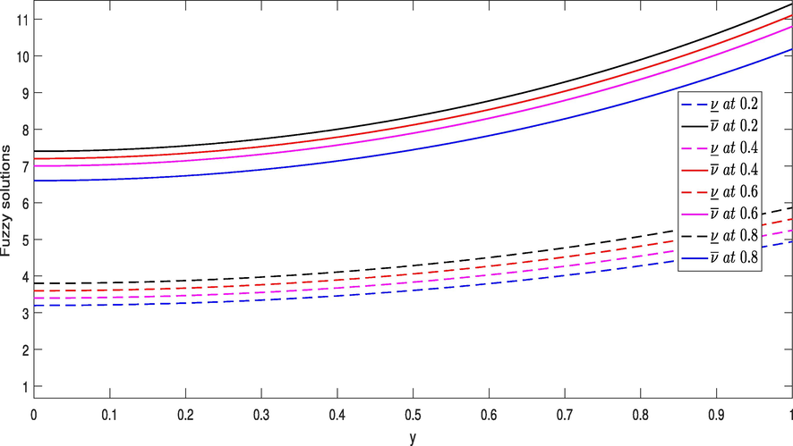
- Graphical presentation of fuzzy solutions at the given values of
for Example 1.
To solve the Eq. (19) by LADM.
Considered the parametric form of Eq. (19) which is given by
Applying the Laplace transform together with convolution Theorem 2 and after the inverse Laplace transform, we get
Let the solution of Eq. (19) in the form of infinite series as
Putting Eq. (22) in Eq. (21), one has
Comparing termwise of Eq. (23) both side respectively
the remaining terms may be in same way computed. The general terms are written as
Taking first lower limit fuzzy solution of Eq. (19), and simplify, one gets
Suppose the following fuzzy linear Volterra integral equation (Salahshour and Allahviranloo, 2013)
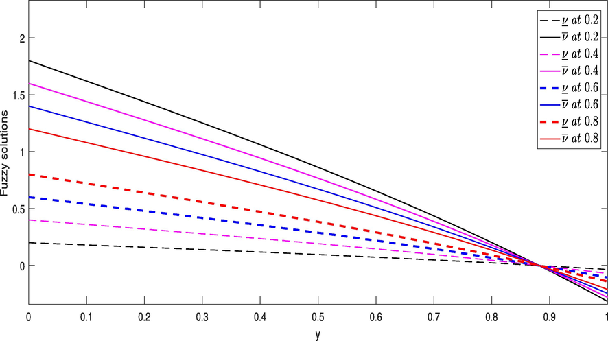
- Graphical presentation of fuzzy solutions at the given values of
for Example 2.
Applying the Laplace transform together with convolution Theorem 2 and the inverse Laplace transform, we obtain
Eq. (27) has solution in the form of series as
Putting Eq. (29) in Eq. (28),
Comparing terms of Eq. (30) on both side respectively, we get
and so on.
Taking first lower limit solution of Eq. (27), and simplify
The remaining terms can be in similarly computed. Putting Eqs. (32) and (33) in Eq. (29) and simplify, we get
Further in more simplified form, we have
Which is the exact solution of the give problem in closed form. Next in Fig. 3, we provide graphical presentation of fuzzy solutions at the given values of uncertainty as
Here we state that in the above test problems, Examples 1 and 2 have been solved numerically by least square method in Ameri and Nezhad (2017). The concerned method is purely a numerical procedure whose convergence is slower than LADM which rapidly converges to exact solution of the problem. Further the Example 3 has been solved in Salahshour and Allahviranloo (2013) by using fractional differential transform method (FDTM) and the same results were achieved as we have got by the proposed method. The one thing which makes LADM more papular is its simplicity in applications while FDTM is slightly complicated in using. Further the convergence rate of the proposed method is faster than differential FDTM (Naghipour and Manafian, 2015).
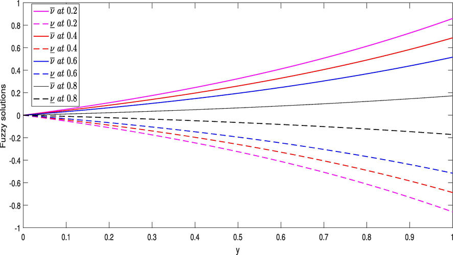
- Graphical presentation of fuzzy solutions at the given values of
for Example 3.
5 Conclusion
In this manuscript, we successfully handled series type analytical solutions to “fuzzy Volterra integral equations” corresponding to separable type kernels. For the required purposes we adopted “LADM” and developed two sequences of upper and lower limit solutions as general algorithm. Then we have tested our proposed scheme on three different problems. Also we stressed that the same solution may be computed in more easy way instead of using complicated method. From the results we concluded that LADM can be applied as a powerful tool in solving both linear and nonlinear problems of fuzzy integral equations. In future work, this method will be applied to investigate the solutions of fuzzy Fredholm and Volterra non-linear integral equations with different kind of crisp and fuzzy kernels.
Declaration of Competing Interest
The authors declare that they have no known competing financial interests or personal relationships that could have appeared to influence the work reported in this paper.
Acknowledgements
The third author would like to thank Prince Sultan University for funding this work through research group Nonlinear Analysis Methods in Applied Mathematics (NAMAM) group number RG-DES-2017-01-17.
References
- Numerical method for solving linear Fredholm fuzzy integral equations of the second kind. Chaos Soliton Fract.. 2007;31:138-146.
- [Google Scholar]
- Fractional operators with generalized Mittag-Leffler kernels and their differintegrals. Chaos. 2019;29:023102
- [CrossRef] [Google Scholar]
- A novel method for a fractional derivative with non-local and non-singular kernel. Chaos, Solitons Fract.. 2018;114:478-482.
- [Google Scholar]
- Solutions of the linear and nonlinear differential equations within the generalized fractional derivatives. Chaos: Interdiscip. J. Nonlinear Sci.. 2019;29(2):023108
- [Google Scholar]
- Solutions of fractional gas dynamics equation by a new technique. Math. Methods Appl. Sci.. 2019;43(3):1349-1358.
- [Google Scholar]
- Existance of global solutions to nonlinear fuzzy Volterra integrao-differential equations. Nonlinear Anal. Theory Methods Appl.. 2012;75:1810-1821.
- [Google Scholar]
- Numerical solution of fuzzy Volterra integral equations based on Least Squares Approximation. ICIC Int.. 2017;11:1451-1460.
- [Google Scholar]
- Atangana, Abdon, 2017. Fractal-fractional differentiation and integration: Connecting fractal calculus and fractional calculus to predict complex system, 102, 396–406.
- Blind in a commutative world: Simple illustrations with functions and chaotic attractors. Chaos, Solitons Fract. 2018;114:347-363.
- [Google Scholar]
- Fractional discretization: The African’s tortoise walk. Chaos, Solitons Fract.. 2020;130:109399
- [Google Scholar]
- Can transfer function and Bode diagram be obtained from Sumudu transform. Alexandria Eng. J. 2020
- [Google Scholar]
- New fractional derivative with non-local and non-singular kernel. Thermal Sci.. 2016;20:757-763.
- [Google Scholar]
- Decolonisation of fractional calculus rules: Breaking commutativity and associativity to capture more natural phenomena. Eur. Phys. J. Plus. 2019;133(4):166.
- [Google Scholar]
- Fractional calculus with power law: The cradle of our ancestors. Eur. Phys. J. Plus. 2019;134(9):429.
- [Google Scholar]
- Chaos in a simple nonlinear system with Atangana-Baleanu derivatives with fractional order. Chaos, Solitons Fract.. 2019;89:447-454.
- [Google Scholar]
- Modeling attractors of chaotic dynamical systems with fractal-fractional operators. Chaos, Solitons Fract.. 2019;123:320-337.
- [Google Scholar]
- A computational method for fuzzy Volterra-Fredholm integral equations. Fuzzy Inf. Eng.. 2011;2:147-156.
- [Google Scholar]
- Numerical solution of linear Fredholm fuzzy integral equations of the second kind by Adomian method. Appl. Math. Comput.. 2005;161:733-744.
- [Google Scholar]
- Quadrature rule for integrals of fuzzy-number-valued function. Fuzzy Set. Syst.. 2004;145:359-380.
- [Google Scholar]
- One-sided fuzzy numbers and applications to integral equations from epidemiology. Fuzzy Sets Syst.. 2013;219:27-48.
- [Google Scholar]
- Open fuzzy cubature rule with application to nonlinear fuzzy Volterra integral equations in two dimensions. Fuzzy Sets Syst.. 2019;358:108-131.
- [Google Scholar]
- A new definition of fractional derivative without singular kernel. Progr. Fract. Differ. Appl.. 2015;1:73-85.
- [Google Scholar]
- On the integrals, series and integral equations of fuzzy set-valued function. J. Harbin Inst. Technol.. 1990;21:11-19.
- [Google Scholar]
- Numerical methods for calculating the fuzzy integral. Fuzzy Set. Syst.. 1996;83:57-62.
- [Google Scholar]
- On typical values and fuzzy integral. IEEE Trans. Syst., Man, Cybernet, Part B. 1997;27:703-705.
- [Google Scholar]
- Numerical solution of fuzzy differential and integral equations. Fuzzy Set. Syst.. 1999;106:35-48.
- [Google Scholar]
- Duality for a class of fuzzy nonlinear optimization problem under generalized convexity. Fuzzy Optim. Decis. Making.. 2014;13:131-150.
- [Google Scholar]
- Kilbas, A., Srivastava, H.M., Trujillo, J.J., 2006. Theory and Application of Fractional Differential Equations, North Holland Mathematics Studies 204.
- Maltok, M., 1987. On fuzzy integrals, in: Proc. 2nd Polish Symp. on interval and Fuzzy Mathematics, Politechnika Poznansk, pp. 167–170.
- An analytical method for solving Fredholm fuzzy integral equations of the second kind. Comput. Math. Appl.. 2011;61:2754-2761.
- [Google Scholar]
- Application of the Laplace Adomian decomposition and implicit methods for solving Burgers’ equation. J. Pure Appl. Math.. 2015;6(1):68-77.
- [Google Scholar]
- Numerical Methods for Fractional Differentiation. Singapore: Springer; 2019.
- On the existence and uniqueness of solutions of fuzzy Volterra-Fredholm integral equations. Fuzzy Sets Syst.. 2000;115(3):425-431.
- [Google Scholar]
- Existence of solutions of fuzzy integral equations in Banach spaces. Fuzzy Set. Syst.. 1995;72:373-378.
- [Google Scholar]
- Existence and uniquencess theorem for a solution of fuzzy Volterra integral equations. Fuzzy Sets Syst.. 1999;105:481-488.
- [Google Scholar]
- Effects of vaccination on measles dynamics under fractional conformable derivative with Liouville-Caputo operator. Eur. Phys. J. Plus. 2020;135(1):63.
- [Google Scholar]
- Mathematical analysis of dengue fever outbreak by novel fractional operators with field data. Physica A. 2019;526:121-127.
- [Google Scholar]
- Fractional modeling for a chemical kinetic reactionin a batch reactor via nonlocal operator with power law kernel. Phys. A: Stat. Mech. Appl.. 2020;542:123494
- [Google Scholar]
- Using Shehu integral transform to solve fractional order Caputo type initial value problems. J. Appl. Math. Comput. Mech.. 2019;18(2):75-83.
- [Google Scholar]
- Monotonically decreasing behavior of measles epidemic well captured by Atangana-Baleanu-Caputo fractional operator under real measles data of pakistan. Chaos, Solitons Fract.. 2020;131:109478
- [Google Scholar]
- Strange chaotic attractors under fractal-fractional operators using newly proposed numerical methods. Eur. Phys. J. Plus. 2019;134(10):523.
- [Google Scholar]
- A new Bernoulli wavelet method for accurate solutions of nonlinear fuzzy Hammerstein-Volterra delay integral equations. Fuzzy Sets Syst.. 2017;309:131-144.
- [Google Scholar]
- Application of fuzzy differential transform method for solving fuzzy Volterra integral equations. Appl. Math. Model.. 2013;37:1016-1027.
- [Google Scholar]
- Application of fuzzy differential transform method for solving fuzzy Volterra integral equations. Appl. Math. Model.. 2013;37:1016-1027.
- [Google Scholar]
- Solving fuzzy integral equations of the second kind by Laplace transform method. Int. J. Ind. Math.. 2012;4(1):21-29.
- [Google Scholar]
- Existence and comparison theorems to Volterra fuzzy integral equation in (En, D)1. Fuzzy Sets Syst.. 1999;104(2):315-321.
- [Google Scholar]
- A note on fuzzy Volterra integral equations. Fuzzy Sets Syst.. 1996;81(22):237-240.
- [Google Scholar]
- The improper fuzzy Riemann integral and its numerical integration. Inform. Sci.. 1999;111:109-137.
- [Google Scholar]
- The fuzzy Riemann integral and its numerical integration. Fuzzy Set. Syst.. 2000;110:1-25.
- [Google Scholar]


