

Translate this page into:
A discussion on controllability of nonlocal fractional semilinear equations of order with monotonic nonlinearity
⁎Corresponding author. msajd@qu.edu.sa (Mohammad Sajid),
-
Received: ,
Accepted: ,
This article was originally published by Elsevier and was migrated to Scientific Scholar after the change of Publisher.
Peer review under responsibility of King Saud University.
Abstract
In this article, we use the tool of monotone nonlinearity to present the approximate controllability discussion for fractional semilinear system with nonlocal conditions. Monotonicity is an important characteristic in many communications applications in which digital-to-analog converter circuits are used. Such applications can function in the presence of nonlinearity, but not in the presence of non-monotonicity. Therefore, it becomes quite interesting to study a problem assuming monotonicity of the nonlinear function. Also, nonlocal conditions are additional specifications for the physical measurements than classical ones and impart a finer effect on the solution. We formulate the control function for the problem and establish the controllability results. At last, we proposed two applications for the demonstration.
Keywords
Monotone condition
Controllability
Mild solution
Fractional order system
Nonlocal conditions
34K30
34K35
93C25

1 Introduction
In the modern years, fractional calculus has been receiving considerable observation from researchers because of its uses in science and engineering areas, such as fractional biological neurons, fractal theories, nonlinear oscillation of earthquake, neural network modeling, fluid dynamics, population dynamics, etc. Fractional Calculus is a very effective mechanism that has been recently incorporated to model complex biological systems with non-linear behavior and long-term memory. It came into picture with a simple question related to the derivation concept like if the first order derivative represents the slope of a function, what would a half order derivative of a function represent? Looking for such type of questions gave birth to many new problems and interesting results in the real world. For example, we cannot determine the properties of a shape memory polymers model by making use of differential frameworks of integer order because the shape varies quickly as there is a small change in the temperature. Therefore, the task of fractional calculus becomes essential here. Fractional calculus has several uses in image processing, oil reservoirs, MRI, gas transportation, damping, HIV/TB infections, etc. So, recently, many researchers have done valuable performances in electromagnetic, control theory, signal, porous media, viscoelasticity, biological, engineering problems, image processing, fluid flow, diffusion, theology, etc. For more specifics, see (Bajlekova et al., 2001; Kilbas et al., 2006; Miller et al., 1993; Podlubny et al., 1999).
On the contrary, controllability problems have fascinated several engineers, mathematicians, and physicists, and remarkable support has been made to theories as well as their application sides also. The controllability of dynamical frameworks under the control of partial differential frameworks has evolved into a widely researched topic in the last three decades. It investigates the probability of driving a system from any starting position to the required terminal position employing some group of admissible controls. Naito (Naito, 1987) obtained the approximate controllability discussion for a semilinear framework governed by linear part utilizing the fixed point technique. For second-order differential systems (Shukla and Patel, 2021; Vijayakumar, 2018; Vijayakumar and Dineshkumar, 2021; Vijayakumar, 2019; Vijayakumar et al., 2017; Vijayakumar et al., 2021; Vijayakumar et al., 2021), and fractional order frameworks have been extensively analyzed in the literature, see, for instance, (Arora, 2018; Arora, 2019; Dineshkumar et al., 2021; Kavitha et al., 2022; Kavitha et al., 2021; Raja et al., 2022; Raja et al., 2021; Nisar and Vijayakumar, 2021; Shukla et al., 2015; Shukla et al., 2014; Shukla et al., 2022; Shukla et al., 2015; SSakthivel and Y.;thivel and Y.; Mahmudov, 2011; Williams et al., 2020; Zhou et al., 2017; Vijayakumar et al., 2013).
Moreover, there are several real world models which can be displayed more accurately as certain partial differential equation with nonlocal conditions. In such problems nonlocal conditions are imposed in place of classical description of the data. These conditions, given by Byszewski (1991), provide excellent results in terms of existence, uniqueness and controllability analysis. It appears mainly when the measurements are considered at regular time periods instead of historical time period. Thus, the investigation may be presented more practically than utilizing the classical condition alone. The controllability problems with nonlocal conditions can be found in Vijayakumar and Dineshkumar (2021).
In SSakthivel and Y.;thivel and Y.; Mahmudov (2011), Sakthivel et al. analyzed the controllability outcomes for semilinear fractional systems by applying theory related to fractional calculus via fixed point approach. Liu and Sakthivel (2014) analyzed the approximate controllability outcomes for semilinear fractional inclusions by applying theory related to fractional calculus via a fixed point approach for multi-valued maps. Zhou (2010) analyzed the existence of fractional neutral differential systems utilizing fixed point theorems and fractional powers of operators. The fundamental theories about the cosine and sine family (CF and SF) for second-order abstract Cauchy problem were introduced by Fattorini et al. (1985) and Travis (1978).
Several authors have focused the approximate controllability discussion about semilinear fractional systems by applying Lipschitz continuity on the nonlinear term with the fixed point technique. Suppose the nonlinear part fulfills monotone condition, then one may get finer conclusions as monotonicity is the main feature of many communication problems. George et al. (1995) and George et al. (1995) established the approximate controllability results for non autonomous semi linear and nonlinear evolution systems with the use of monotone and integral contractor condition on the nonlinear term. Arora (2019) discussed the controllability outcomes for fractional frameworks of order with nonlinear term possess integral contractor. But no results are dealing with the nonlocal fractional semi linear control system of order using monotone condition on the nonlinear term.
Let
and
be the function spaces defined on
, where
and
are two Hilbert spaces. Consider the following nonlocal fractional semi linear control system:
-
is the Caputo fractional derivative of order .
-
represents the state having values in Hilbert space .
-
Control function v is defined from .
-
is a bounded linear operator.
-
The map produces nonlinearity in the system.
-
The operator is linear, closed where is a dense subset of .
-
h and are continuous functions from .
The fractional linear system with nonlocal conditions associated with (1.1)–(1.3) along with control u is presented as
2 Auxiliary results
We recollect known essential facts, lemmas, elementary definitions, remarks, and outcomes related to fractional calculus, semigroup theory of linear operators, and control theory.
We assume that stand for the space of functions that are continuous and 1-time continuously differentiable. Here denotes the set of bounded linear operators from the Hilbert space to .
(Kilbas et al., 2006) “Provided that , then the Riemann–Liouville (R-L) fractional integral of order is presented as In the above, .”
(Kilbas et al., 2006) “The R-L fractional derivative for of order is presented as
(Kilbas et al., 2006) “The Caputo fractional derivative of order is presented as where .”
Assume that the subsequent fractional evolution system:
(Bajlekova et al., 2001) “Assume that . A family is said to be a solution operator (or a strongly continuous r-order fractional CF) for (2.1) provided that the subsequent characteristics are fulfilled:
-
is strongly continuous for and .
-
such that .
-
and .
-
is a solution for (2.1), .”
A is said to be infinitesimal generator of . The strongly continuous r-order fractional CF is also said to be r-order CF.
The fractional SF connected with is presented as
The fractional R-L family connected with is presented as
Now, using the definition of R-L integral, we obtain for , Next, we describe the mild solution for (1.1)–(1.3) and its corresponding linear system.
The mild solution of (1.1)–(1.3) is defined by which satisfy the following integral equation. and the mild solution for (1.4)–(1.6) is described by the following integral equation
(Curtain et al., 1995) “The system (1.1)–(1.3) is said to be approximately controllable in , provided that for given starting position and required final position and a control function such that the solution of (1.1)–(1.3) fulfills where is the state value of (1.1)–(1.3) at time .”
Suppose , then the system is called exactly controllable.
Controllability can also be interpreted in terms of reachable set which is defined in the following manner.
(Curtain et al., 1995) “Reachable set is the collection of all the possible final positions corresponding to the control . The set defined by is the reachable set for (1.1)–(1.3) and is the reachable set for (1.4)–(1.6).”
(Curtain et al., 1995) Definition of Approximate Controllability in terms of Reachable Set: “A control system is said to be approximately controllable on an interval , iff the corresponding reachable set is dense in . Therefore the given system (1.1)–(1.3) is approximately controllable iff where denotes the closure of .
If , then the given system is said to exactly controllable.”
3 Controllability results
Here we mainly focus on the controllability for the second order fractional semilinear control system with nonlocal conditions considering the monotone nonlinearity of the nonlinear term.
The following conditions are taken into account to obtain the approximate controllability results of (1.1)–(1.3):
-
a constant such that where is the operator defined by
-
Linear fractional system with nonlocal conditions (1.4)–(1.6) is approximately controllable, that is, the corresponding reachable set is dense in .
-
Monotone condition is satisfied by the nonlinear function , that is, constant such that
-
, where and are constants and is Nemytskii operator defined as
-
, that is, for any given a w in such that
(3.1) -
There exist constants and such that and .
The solution of the nonlocal fractional system (1.1)–(1.3) connected with the control fulfills the subsequent where for each .
Let be the mild solution of (1.1)–(1.3) associated with the control . Therefore, one can consider in the following way: Taking norm on both sides, we get Applying Gronwall’s inequality, we attain Hence, the result is proved.
Suppose that - are fulfilled, then the fractional semilinear control system with nonlocal conditions (1.1)–(1.3) is approximately controllable on .
Assume that
be the mild solution of the fractional linear system with nonlocal conditions (1.4)–(1.6) associated with the control u. Then we can write
as
If we can show that is negligbly small, then it will indicate that is also arbitrary small from the Eq. (2.5).
Therefore, we show that is arbitrarily small.
Using Cauchy Schwartz Inequality, we have
Now, using Eqs. (2.5), (2.6)condition , we get that , for some .
Next, we determine that is arbitrary small.
Consider,
Thus, we get
(reachable set for the fractional semilinear control system with nonlocal conditions (1.1)–(1.3) is dense in (corresponding fractional linear system with nonlocal conditions (1.4)–(1.6).
But is dense in due to the condition as the corresponding fractional linear system with nonlocal conditions is approximately controllable. Therefore, is dense in , which implies that (1.1)–(1.3) is approximately controllable.
4 Applications
4.1 Abstract system
Assume the fractional differential system has the form:
Because A is the infinitesimal generator of a strongly continuous CF for . Now, using the subordinate theorem (Bajlekova et al., 2001), which gives A is the infinitesimal generator of a strongly continuous exponentially bounded fractional CF such that , also where , and Let be defined by where be a continuous control function.
Let be defined by where is a nonlinear function.
We now define in the following way: for .
Here, the nonlinear function can be considered satisfying the conditions - . The nonlocal functions and can be taken satisfying the assumption .
The problem (4.1)–4.4 can be rewritten as Therefore, by Theorem 3.1, the fractional differential system (4.1)–(4.4) is approximately controllable.
4.2 Filter system
Digital filters (DFs) play an extremely important role in the field of Digital Signal Processing (DSP). The execution of DFs is phenomenal; each of the critical factors that DSP has grown highly regarded. Filters are commonly classified as having two main applications: signal separation and signal restoration.
If a transmission is influenced by agitation, sound disturbance, or other signals, the use of filters in signal separation is essential. For instance, if one gadget is used to calculate the electrical operation of a baby’s heart (EKG) while still in the womb. Using a mother’s breath and pulse as a coarse indicator could be humiliating. To separate these signals from the target, a filter might be used.
We provide our filter system Fig. 1 as a response to the Filter systems presented in Zahoor et al. (2017) and Chandra et al. (2016). Fig. 1 depicts the block diagram’s rough layout, which aids in improving the solution’s utility while using the smallest amount of inputs possible. (i) Product modulator (PM)-1 accepts the input
and A gives an output of
. Likewise, (ii) PM-2 accepts
and
produces
, (iii) PM-3 accepts
and B gives
, (iv) PM-4 accepts
and
at time
, produces
, (v) PM-5 accepts
and
at time
, produces
, respectively. The integrators execute the integral of
, over the period
.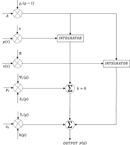
Filter System.
Finally, we move the outputs from the integrators to the summer network. Therefore, the output of is attained, it is bounded and approximately controllable.
5 Conclusion
In the present manuscript, we have established the approximate controllability results for nonlocal fractional semilinear system with order . The results have been determined by assuming the monotone condition on the nonlinear term.
The method discussed in the present article can be further utilized to discuss the approximate controllability results for nonlocal impulsive fractional system after suitable modifications.
Acknowledgments
The researchers would like to thank the Deanship of Scientific Research, Qassim University for funding the publication of this project.
Declaration of Competing Interest
The authors declare that they have no known competing financial interests or personal relationships that could have appeared to influence the work reported in this paper.
References
- Controllability of retarded semilinear fractional system with non-local conditions. IMA J. Math. Control Inform.. 2018;35(3):689-705.
- [CrossRef] [Google Scholar]
- Controllability of fractional system of order r∈(1,2] with nonlinear term having integral contractor. IMA J. Math. Control Inform.. 2019;36(1):271-283.
- [CrossRef] [Google Scholar]
- Fractional evolution equations in Banach spaces, Eindhoven University of Technology. Eindhoven 2001
- [CrossRef] [Google Scholar]
- Theorem about the existence and uniqueness of a solution of a nonlocal abstract Cauchy problem in a Banach space. Appl. Anal.. 1991;40(1):11-19.
- [CrossRef] [Google Scholar]
- Design of hardware efficient FIR filter: a review of the state of the art approaches. Eng. Sci. Technol., Int. J.. 2016;19:212-226.
- [CrossRef] [Google Scholar]
- Curtain, R.F.; Zwart, H.J.; An Introduction to Infinite Dimensional Linear Systems Theory, Springer Verlag, New York, (1995). https://doi.org/10.1007/978-1-4612-4224-6
- A note on the approximate controllability of Sobolev type fractional stochastic integro-differential delay inclusions with order 1< r< 2. Math. Comput. Simulat.. 2021;190:1003-1026.
- [CrossRef] [Google Scholar]
- Second order linear differential equations in Banach spaces, North-Holland Mathematics Studies, 108. Amsterdam: North-Holland Publishing Co.; 1985.
- Approximate controllability of nonautonomous semilinear systems. Nonlinear Anal.. 1995;24(9):1377-1393.
- [Google Scholar]
- Approximate controllability of semilinear systems using integral contractors. Numer. Funct. Anal. Optim.. 1995;16(1–2):127-138.
- [Google Scholar]
- Results on controllability of Hilfer fractional differential equations with infinite delay via measures of noncompactness. Asian J. Control. 2022;24(3):1406-1415.
- [CrossRef] [Google Scholar]
- Results on approximate controllability of Sobolev-type fractional neutral differential inclusions of Clarke subdifferential type. Chaos Solitons Fractals. 2021;151(1–8):111264
- [CrossRef] [Google Scholar]
- Theory and applications of fractional differential equations, North-Holland Mathematics Studies, 204. Amsterdam: Elsevier; 2006.
- Approximate controllability of fractional functional evolution inclusions with delay in Hilbert spaces. IMA J. Math. Control Inform.. 2014;31(3):363-383.
- [CrossRef] [Google Scholar]
- An introduction to the fractional calculus and fractional differential equations. Wiley, New York: A Wiley-Interscience Publication; 1993.
- Optimal control and approximate controllability for fractional integrodifferential evolution equations with infinite delay of order r ∈(1,2) Optim. Control Appl. Methods 2022:1-24.
- [CrossRef] [Google Scholar]
- New discussion on nonlocal controllability for fractional evolution system of order 1< r< 2. Adv. Difference Eqs.. 2021;2021(1):1-19.
- [CrossRef] [Google Scholar]
- Controllability of semilinear control systems dominated by the linear part. SIAM J. Control Optimiz.. 1987;25:715-722.
- [CrossRef] [Google Scholar]
- Results concerning to approximate controllability of non-densely defined Sobolev-type Hilfer fractional neutral delay differential system. Math. Methods Appl. Sci.. 2021;44(17):13615-13632.
- [CrossRef] [Google Scholar]
- differential equations, Mathematics in Science and Engineering, 198. CA: Academic Press, San Diego; 1999.
- On the approximate controllability of semilinear fractional differential systems. Comput. Math. Appl.. 2011;62(3):1451-1459.
- [CrossRef] [Google Scholar]
- Complete controllability of semi-linear stochastic system with delay. Rendiconti del Circolo Matematico di Palermo. 2015;64:209-220.
- [CrossRef] [Google Scholar]
- Controllability of semilinear stochastic system with multiple delays in control. IFAC Proc.. 2014;47(1):306-312.
- [CrossRef] [Google Scholar]
- Existence and optimal control results for second-order semilinear system in Hilbert Spaces. Circuits Syst. Signal Process. 2021;40:4246-4258.
- [CrossRef] [Google Scholar]
- A new exploration on the existence and approximate controllability for fractional semilinear impulsive control systems of order r ∈(1, 2) Chaos Solitons Fractals. 2022;154(1–8):111615
- [CrossRef] [Google Scholar]
- Approximate controllability of semilinear stochastic control system with nonlocal conditions. Nonlinear Dyn. Syst. Theory. 2015;15(3):321-333.
- [CrossRef] [Google Scholar]
- Cosine families and abstract nonlinear second order differential equations. Acta Mathematica Academiae Scientiarum Hungaricae. 1978;32(1–2):75-96.
- [CrossRef] [Google Scholar]
- Approximate controllability of second order nonlocal neutral differential evolution inclusions. IMA J. Math. Control Inform.. 2021;38(1):192-210.
- [CrossRef] [Google Scholar]
- Controllability for a class of second-order evolution differential inclusions without compactness. Appl. Anal.. 2019;98(7):1367-1385.
- [CrossRef] [Google Scholar]
- Approximate controllability results for abstract neutral integro-differential inclusions with infinite delay in Hilbert spaces. IMA J. Math. Control Inform.. 2018;35(1):297-314.
- [CrossRef] [Google Scholar]
- Controllability of second order impulsive nonlocal Cauchy problem via measure of noncompactness. Mediterr. J. Math.. 2017;14(1):1-22.
- [CrossRef] [Google Scholar]
- Results on approximate controllability results for second-order Sobolev-type impulsive neutral differential evolution inclusions with infinite delay. Numer. Partial Diff. Eqs.. 2021;37(2):1200-1221.
- [CrossRef] [Google Scholar]
- Nonlocal controllability of mixed Volterra-Fredholm type fractional semilinear integro-differential inclusions in Banach spaces. Dyn. Continuous, Discrete Impuls. Syst.. 2013;20(4–5b):485-502.
- [Google Scholar]
- Approximate controllability of second order nonlocal neutral differential evolution inclusions. IMA J. Math. Control Inform.. 2021;38(1):192-210.
- [CrossRef] [Google Scholar]
- Existence and controllability of nonlocal mixed Volterra-Fredholm type fractional delay integro-differential equations of order 1<r<2. Numerical Methods for Partial Differential Equations 2020:1-21.
- [CrossRef] [Google Scholar]
- Design and implementation of an efficient FIR digital filter. Cogent Eng.. 2017;4(1):1-13. 1323373
- [CrossRef] [Google Scholar]
- Controllability results for fractional order neutral functional differential inclusions with infinite delay. Fixed Point Theory. 2017;18(2):773-798. https://doi.org/10.24193/fpt-ro.2017.2.62
- [Google Scholar]
- Existence of mild solutions for fractional neutral evolution equations. Comput. Math. Appl.. 2010;59(3):1063-1077.
- [CrossRef] [Google Scholar]


