

Translate this page into:
A bounded distribution derived from the shifted Gompertz law
⁎Address: María de Luna 3, 50018 Zaragoza, Spain. pjodra@unizar.es (P. Jodrá)
-
Received: ,
Accepted: ,
This article was originally published by Elsevier and was migrated to Scientific Scholar after the change of Publisher.
Abstract
A two-parameter probability distribution with bounded support is derived from the shifted Gompertz distribution. It is shown that this model corresponds to the distribution of the minimum of a random number with shifted Poisson distribution of independent random variables having a common power function distribution. Some statistical properties are written in closed form, such as the moments and the quantile function. To this end, the incomplete gamma function and the Lambert W function play a central role. The shape of the failure rate function and the mean residual life are studied. Analytical expressions are also provided for the moments of the order statistics and the limit behavior of the extreme order statistics is established. Moreover, the members of the new family of distributions can be ordered in terms of the hazard rate order. The parameter estimation is carried out by the methods of maximum likelihood, least squares, weighted least squares and quantile least squares. The performance of these methods is assessed by means of a Monte Carlo simulation study. Two real data sets are used to illustrate the usefulness of the proposed distribution.
Keywords
Bounded distribution
Shifted Gompertz
Beta
Kumaraswamy
Power function
60E05
62P10
33B30

1 Introduction
Over the last decades, there has been considerable interest in the development of new parametric probability distributions, which can be used in a wide range of practical applications. Almost all new proposals are distributions with unbounded support. However, there are many real situations in which the data take values in a bounded interval, such as percentages and proportions. The most popular two-parameter distributions with bounded support are the classical beta and Kumaraswamy laws (for the latter see Kumaraswamy, 1980, Jones, 2009). Other less known models are the transformed Leipnik distribution (Jorgensen, 1997, pp. 196–197), the Log–Lindley distribution (Gómez-Déniz et al., 2014; Jodrá and Jiménez-Gamero, 2016) and the standard two-sided power distribution (Van Dorp and Kotz, 2002). In the mathematical literature, there are proposals with more parameters such as the three-parameter generalized beta distribution (McDonald, 1984) and the reflected generalized Topp–Leone power series distribution (Condino and Domma, 2017), the four-parameter Kumaraswamy Weibull distribution (Cordeiro et al., 2010), the exponentiated Kumaraswamy-power function distribution (Bursa and Ozel, 2017) and the two-sided generalized Kumaraswamy distribution (Korkmaz and Genç, 2017) and the five-parameter Kumaraswamy generalized gamma distribution (Pascoa et al., 2011), among others, but in these cases their handling is more complex due to the greater number of parameters. The usefulness of distributions with bounded support has been highlighted in Condino and Domma (2017), Cordeiro et al. (2010), Kotz and van Dorp (2004), Pascoa et al. (2011) and the references therein.
In this paper, our proposal is to provide a new two-parameter distribution for modelling data taking values in a bounded domain. Specifically, a new random variable defined on the interval (0,1) is derived from the shifted Gompertz (SG) distribution. The SG law was introduced by Bemmaor (1994) as a model of adoption timing of a new product in a marketplace, showing its connection with the Bass diffusion model widely used in marketing research (see Bemmaor and Lee, 2002). The properties of the SG distribution were throughly studied in Jiménez and Jodrá (2009) and the parameter estimation in Jiménez (2014), Jukić and Marković (2017).
To start with, let Y be a random variable having a SG distribution with parameters
and
, whose cumulative distribution function (cdf) is given by
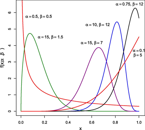
for different values of
and
.
It should be noted that the standard power function distribution with parameter is obtained by setting in (2); in particular, the case and corresponds to the uniform distribution. Since the power function distribution is a well-studied model, for the sake of simplicity the special case has been intentionally omitted in the current study.
Note also that the LSG law defined by (2) in the unit interval can be extended to any bounded domain in a straightforward manner, since a linear transformation moves a random variable X defined on to any other bounded support , with . Accordingly, there is no need to study such an extension further.
The remainder of this paper is organized as follows. In Section 2, some statistical properties of the LSG distribution are studied. First, a stochastic representation is given. Next, the moments are expressed in closed form in terms of the incomplete gamma function and the quantile function is written in terms of the Lambert W function. The shape of the failure rate function and the mean residual life are also studied. Analytical expressions are provided for the moments of the order statistics and the limit behavior of the extreme order statistics is established. It is also shown that the members of the new family of distributions can be ordered in terms of the hazard rate order. In Section 3, the parameter estimation is carried out by maximum likelihood, least squares, weighted least squares and quantile least squares. A Monte Carlo simulation study assesses the performance of these methods. Finally, in Section 4, two real data sets illustrate that the LSG model may provide a better fit than other two-parameter distributions with bounded support.
2 Statistical properties
2.1 Stochastic representation
The LSG distribution has been defined in (2) via an exponential transformation of the SG model. It is interesting to note that the LSG law can be obtained as the distribution of the minimum of a shifted Poisson random number of independent random variables having a common power function distribution. To be more precise, let N be a random variable having a Poisson distribution with mean , so its probability mass function is given by Let M be a shifted Poisson random variable defined by . Let be independent identically distributed random variables having a standard power function distribution with parameter , that is, its cdf is . Assume also that M is independent of , for .
The random variable has a distribution.
For any and , the conditional cdf of the random variable is given by . Therefore, Hence, for any and the marginal cdf of T is given by which implies the result. □
As contexts of potential application of the LSG distribution, note that in medical and veterinary studies a patient/animal may die due to different unknown causes such as infections. In this context, M denotes the number of causes and denotes the lifetime in a bounded period associated with each cause i. In the described scenario, frequently only the minimum lifetime T among all causes will be observed. A similar scenario can be found in reliability, where a complex device may fail due to different unknown causes.
2.2 Shape and mode
The next result describes the different shapes of pdf (2) depending on the values of the parameters. The proof is omitted because it consists of routine calculations.
Let X be a random variable having a distribution.
-
For any and is a decreasing function in x.
-
For any and , is an increasing function in x.
-
For any and , has a mode given by Morover, for any and for any and .
From Proposition 2.2, a clear difference between the LSG law and the beta and Kumaraswamy distributions is the limit behavior at , since that limit can be equal to 0, 1 or in the beta and Kumaraswamy models.
2.3 Moments
The moments of the LSG distribution can be expressed analytically in terms of the lower and upper incomplete gamma functions (see Paris, 2010, pp. 174), which are defined, respectively, by
Let X be a random variable having a
distribution. For
, the k-th moment of X is given by
By making the change of variable and taking into account (4), The result follows by applying to the above equation the recurrence formula (Paris, 2010, pp. 178). □
Computer algebra systems usually implement the upper incomplete gamma function instead of the lower one, so it is also useful to express (5) in terms of the former.
Let X be a random variable having a
distribution. For
, the k-th moment of X is given by
The result follows from Eq. (5) together with the fact that (Paris, 2010, pp. 174). □
From Corollary 2.4, the usual statistical measures involving
can be computed efficiently. Figs. 2 and 3 illustrate, respectively, the behavior of the mean and the standard deviation (denoted by
) for different values of the parameters.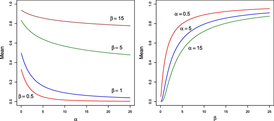
Mean for several values of
and
.
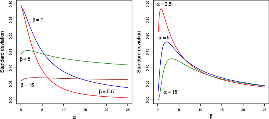
Standard deviation for different values of
and
.
Figs. 4 and 5 display, respectively, the behavior of the asymmetry coefficient,
, and the kurtosis coefficient,
, for different values of the parameters. As can be seen, the LSG distribution has a wide range of values for both coefficients depending on the values of
and
, which suggests that the proposed model is rich enough to model real data.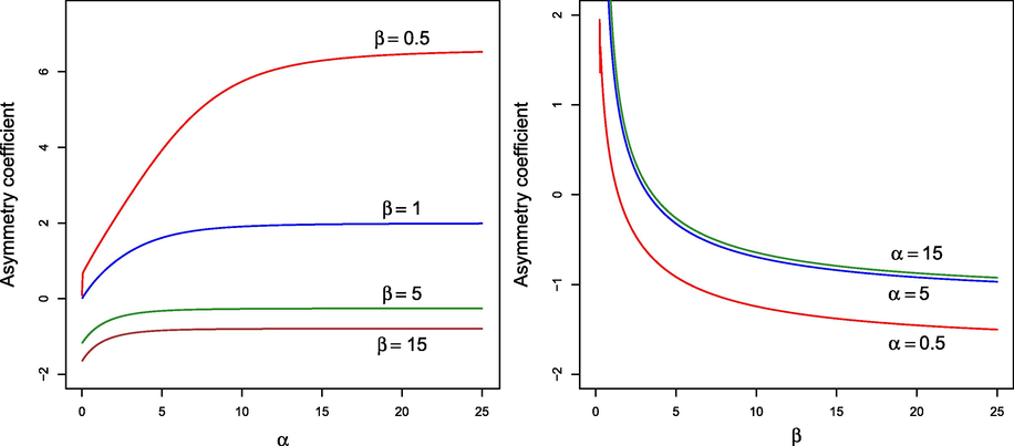
Asymmetry coefficient for different values of
and
.
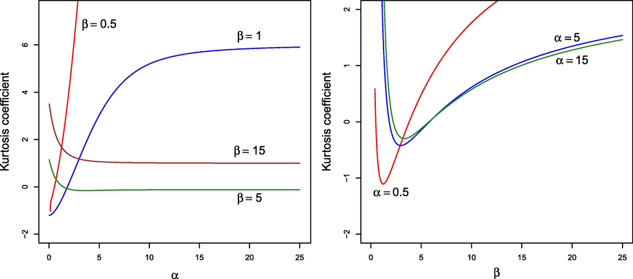
Kurtosis coefficient for different values of
and
.
2.4 Quantile function
An outstanding property of the LSG distribution is that its cdf is invertible. Specifically, the quantile function can be expressed in closed form in terms of the principal branch of the Lambert W function.
For the sake of completeness, recall that the Lambert W function is a multivalued complex function defined as the solution of the equation , where z is a complex number. This function has two real branches if z is a real number such that . The real branch taking on values in (resp. ) is called the principal (resp. negative) branch and is denoted by (resp. ). A review of this special function can be found in the seminal paper by Corless et al. (1996).
The quantile function of the
distribution is given by
For any , we have to solve with respect to x the equation , which is equivalent to solve , with given by Eq. (1). The solution of the latter equation is . Now, by taking into account the closed-form expression for provided in Jiménez and Jodrá (2009, Proposition 3.1), we get which is equivalent to (7). □
For simulation purposes, Proposition 2.5 is very useful because pseudo-random data from the LSG model can be computer-generated from formula (7) in a straightforward manner by applying the inverse transform method (see, for example, Fishman (1996, Chapter 3)). More precisely, a pseudo-random datum from the LSG model is generated evaluating in formula (7) a pseudo-random datum from a uniform distribution defined on (0,1). In this regard, it should be remarked that the Lambert W function is available in computer algebra systems such as Maple (function LambertW), Mathematica (function ProductLog) and Matlab (function lambertw) and in programming languages such as R Development Core Team (2018) (functions lambertW0 and lambertWm1 for and , respectively, in the package lamW).
2.5 Failure rate and mean residual life
The failure (or hazard) rate and the mean residual life are essential in reliability and lifetime data analysis. The failure rate gives a description of the random variable in an infinitesimal interval of time whereas the mean residual life describes it in the whole remaining interval of time.
The failure rate function of the
distribution is given by
(i) If then the LSG law has an increasing failure rate (IFR). (ii) If then there exists so that is (strictly) decreasing when and (strictly) increasing when .
The first derivative of h can be written as below Part (i) follows because for any and . To prove part (ii), let . For any and , note that is an increasing function in x since Moreover, and . As a consequence, there exists such as for and for , which implies the result. □
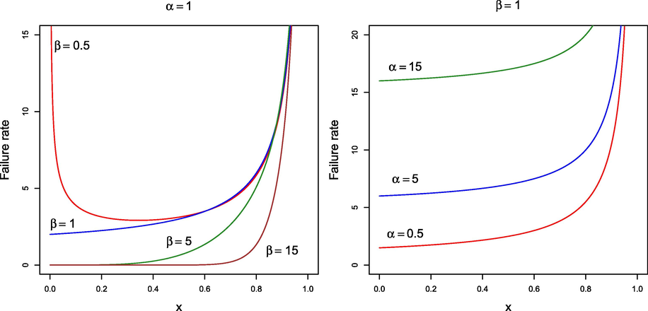
- Failure rate functions for
(left) and
(right).
The different shapes of the failure rate function depending on the values of the parameters suggest a great flexibility of the LSG distribution to model real data.
On the other hand, the mean residual life function is defined by . It is known that if a random variable has an IFR then the mean residual life is decreasing. Therefore, as a consequence of Proposition 2.6, for the LSG distribution has decreasing mean residual life. In the following result, the mean residual life is written in closed form.
For any , the mean residual life of the distribution is given by
Let . For any , we have where we have made the change of variable in the third equality and Eq. (4) was considered in the last one. Finally, the desired result is obtained by taking into account that , and (Paris, 2010, pp. 178). □
2.6 Order statistics
This section provides analytical expressions to compute the moments of the order statistics and also studies the limit behavior of the extreme order statistics.
Let
be n independent random variables having LSG
distribution. Let
be the order statistics obtained by arranging
,
, in non-decreasing order of magnitude. In particular, the minimum
and maximum
are called the extreme order statistics. For any
and
, it is known that the kth moment of
can be computed using the following formula (see, for example, Balakrishnan and Rao, 1998, pp. 7)
For , the k-th moment of the smallest order statistic from the distribution is given by
The result is derived from formula (9) setting , by applying the change of variable , the binomial theorem, the recurrence formula and also that (the details are omitted here). □
The expression of in Proposition 2.8 can be used to compute , for and , avoiding the use of Eq. (9). With this aim, it can be used the recurrence formula (see Balakrishnan and Rao, 1998, pp. 156)
Next, the limit behaviour of the extreme order statistic is established. First, recall that the cdfs of
and
are given, respectively, by
and
, with
defined by (3). When n increases to
, it is well-known that their limit distributions degenerate being needed to apply linear transformations to avoid degeneration. If there exist a non–degenerate cdf H and normalizing constants
and
such that
The distribution belongs to:
Part (i) is a consequence of Arnold et al. (1992, Theorems 8.3.2 and 8.3.4) by taking into account that where from (7) (details of the calculations are omitted here). Similarly, part (ii) is a consequence of Arnold et al. (1992, Theorems 8.3.6) by taking into account that The proof is complete. □
2.7 Stochastic orderings
To conclude Section 2, it is shown that the members of the LSG family can be ordered in terms of the hazard rate order, which is stronger than the usual stochastic order and the mean residual life order. For the sake of completeness these definitions are given below (see Shaked and Shanthikumar, 2007 for more details).
Let and be two random variables with cdfs and , respectively. Let and be the hazard rate functions of and , respectively. Let and be the mean residual life functions of and , respectively.
-
is said to be smaller than in the hazard rate order, denoted by , if for all x.
-
is said to be stochastically smaller than , denoted by , if for all x.
-
is said to be smaller than in the mean residual life order, denoted by , if for all x.
The hazard rate order has applications in reliability theory and life insurance for comparing remaining lifetimes. Given two random variables and representing times until death, means that items with remaining lifetime will tend to live longer that those with remaining lifetime . The LSG family is ordered according to the value of the parameters in the following way.
Let and be two random variables having and distributions, respectively. If then .
From Eq. (8), . The result follows since clearly for any . □
Let and be two random variables having and distributions, respectively. If then the following relations hold:
-
,
-
,
-
for all .
Part (i) follows from the fact that (see Shaked and Shanthikumar, 2007, pp. 18). Part (ii) follows from the property (see Shaked and Shanthikumar, 2007, pp. 83). Part (iii) is a consequence of part (i) and the fact that if and only if for all non-decreasing functions g (see Shaked and Shanthikumar, 2007, pp. 4). □
In particular, Corollary 2.12 shows that, for fixed , the mean of the LSG family decreases as increases.
3 Parameter estimation
The estimation of parameters of the LSG distribution is considered in this section. Initially, the maximum likelihood (ML) method is applied and the performance of this method is assessed via a Monte Carlo simulation study. Asymptotic as well as bootstrap confidence intervals for the model parameters are also discussed. Next, methods based on least squares are applied and their performance evaluated via a simulation study.
3.1 Maximum likelihood method
Let
be a random sample of size n from a
law with both parameters unknown and denote by
, …,
the observed values. From the likelihood function,
, the log-likelihood function is given by
3.1.1 Practical considerations and simulation results
It is clear that the system of Eqs. (13) does not have an explicit solution. Consequently, to obtain the ML estimates it is preferable to solve the following optimization problem
A Monte Carlo simulation study was carried out to evaluate the performance of the ML method. Let N be the number of random samples generated and n the size of each random sample. The following quantities were computed for the simulated estimates :
-
The mean: .
-
The bias: .
-
The mean-square error: .
The quantities and are analogously defined and were also computed.
We generated
random samples of sizes
for different values of
and
. Pseudo-random data from the LSG distribution were computer-generated by using formula (7). Problem (14) was solved using the BFGS algorithm available in the function constrOptim in the R language (R Development Core Team, 2018). Table 1 shows some simulation results, where the mean, bias and MSE of the simulated estimates are reported together with the corresponding asymptotic variances denoted by Var(
) and Var(
). The asymptotic variances were obtained from the diagonal elements of the inverse of the expected Fisher information matrix. In this respect, the expected Fisher information matrix is defined as
, where
is the Hessian matrix of
(see Lehmann and Casella, 1998, for further details). Specifically,
where
As far as we have been able to determine, the integral expressions defining the elements of
cannot be written in closed form and, accordingly, for the particular values of
and
in Table 1 the elements
and
were calculated by numerical integration. The diagonal elements of
provided the variances in Table 1. Note that, alternatively, the asymptotic variances can also be approximated from the diagonal elements of the inverse of the observed Fisher information matrix. The observed information matrix will be provided in the next subsection.
Bias(
)
MSE(
)
Var(
)
Bias(
)
MSE(
)
Var(
)
Bias(
)
MSE(
)
Var(
)
Bias(
)
MSE(
)
Var(
)
0.635
0.1356
0.2647
0.2595
0.524
0.0242
0.0109
0.0109
0.637
0.1372
0.2704
0.2595
5.245
0.2455
1.0987
1.0984
0.558
0.0584
0.1306
0.1297
0.510
0.0107
0.0054
0.0054
0.556
0.0569
0.1317
0.1297
5.103
0.1032
0.5498
0.5492
0.524
0.0241
0.0654
0.0648
0.504
0.0043
0.0027
0.0027
0.529
0.0296
0.0671
0.0648
5.045
0.0455
0.2755
0.2746
0.509
0.0091
0.0263
0.0259
0.501
0.0018
0.0010
0.0010
0.508
0.0087
0.0262
0.0259
5.013
0.0133
0.1119
0.1098
0.503
0.0030
0.0129
0.0129
0.500
0.0005
0.0005
0.0005
0.504
0.0042
0.0130
0.0129
5.008
0.0081
0.0559
0.0549
Bias(
)
MSE(
)
Var(
)
Bias(
)
MSE(
)
Var(
)
Bias(
)
MSE(
)
Var(
)
Bias(
)
MSE(
)
Var(
)
5.505
0.5058
3.3367
2.0388
0.513
0.0136
0.0042
0.0036
11.415
1.4156
17.9270
8.9093
10.310
0.3105
1.5630
1.2876
5.240
0.2403
1.3001
1.0194
0.506
0.0069
0.0020
0.0018
10.619
0.6197
6.0600
4.4546
10.145
0.1454
0.7034
0.6438
5.105
0.1056
0.5638
0.5097
0.502
0.0026
0.0009
0.0009
10.293
0.2934
2.6612
2.2273
10.065
0.0655
0.3399
0.3219
5.049
0.0492
0.2140
0.2038
0.501
0.0012
0.0003
0.0003
10.132
0.1327
0.9432
0.8909
10.029
0.0290
0.1289
0.1287
5.029
0.0291
0.1061
0.1019
0.500
0.0008
0.0001
0.0001
10.052
0.0523
0.4590
0.4454
10.011
0.0117
0.0643
0.0643
Looking at Table 1, it can be noted that the ML method tended to slightly overestimate the value of both parameters. In spite of this fact, the ML method provided acceptable estimates of the parameters. As expected, the bias and MSE decrease as n increases and the values of MSE and variance are, in general, close.
3.1.2 Interval estimation
Based on the asymptotic normal approximation for , interval estimation (similarly hypothesis tests) can be easily performed from the observed information matrix . This matrix is given by where The observed covariance matrix is the inverse of , and the diagonal elements of are the variances of and , which we denote by and , respectively. Then, the asymptotic confidence intervals for and are and , respectively, where stands for the upper percentile of the standard normal distribution.
It is well-known that the confidence intervals based on the asymptotic normal distribution of the ML estimates may not be suitable for samples of small size. To determine in practice for what values of n is observed that normal behavior, we generated 10,000 samples of different sizes n for different values of the parameters. From our simulation experiments, we observed that the approximate normality of the ML estimates requires sample sizes n greater than 1000. This fact was checked by means of histograms, Q-Q plots and normality tests such as Kolomogrov–Smirnov and Anderson–Darling (the details are omitted here).
Accordingly, for samples of size 1000 or smaller we recommend constructing the confidence intervals using other techniques, such as parametric bootstrap. Table 2 shows the coverage probability (CP) and average width (AW) of 95% percentile bootstrap confidence intervals for each parameter. These simulation results were obtained by generating 10,000 samples of different sizes n and considering 1000 bootstrap samples in each case. As can be seen, as the sample size n increases the coverage probabilities are close to the nominal level of 95% and the average widths decrease.
n
CP(
)
AW(
)
CP(
)
AW(
)
0.5
0.5
100
0.9539
1.3154
0.9464
0.2782
200
0.9547
0.9559
0.9447
0.2001
500
0.9469
0.6306
0.9467
0.1296
1000
0.9517
0.4471
0.9508
0.0918
0.5
5.0
100
0.9540
1.3154
0.9464
2.7828
200
0.9575
0.9576
0.9502
2.0012
500
0.9477
0.6310
0.9446
1.2963
1000
0.9505
0.4470
0.9510
0.9183
5.0
0.5
100
0.9335
4.5627
0.9433
0.1730
200
0.9437
2.9945
0.9432
0.1200
500
0.9464
1.8086
0.9450
0.0750
1000
0.9482
1.2635
0.9527
0.0528
10.0
10.0
100
0.9326
10.1106
0.9396
3.2698
200
0.9368
6.4646
0.9401
2.2634
500
0.9431
3.8292
0.9465
1.4116
1000
0.9483
2.653
0.9517
0.9938
3.2 Estimation methods based on least squares
This Section describes the estimation of parameters using the methods of least squares (LS), weighted least squares (WLS) and quantile least squares (QLS). Next, a Monte Carlo simulation study evaluates the performance of these methods.
Before going further, some notation is introduced. Let
be the order statistics of a random sample of size n from a
distribution with both parameters unknown. Denote by
the ordered observed data. It is well-known that the empirical distribution function is considered an estimator of
, which is defined as below
3.2.1 Least squares method
The approach proposed by Bain (1974) was applied to obtain the LSG estimates of the parameters, which are the values
and
that minimize the following least squares function
3.2.2 Weighted least squares method
The parameters of the LSG distribution were also estimated by the WLS method. Following Bickel and Doksum (2001, pp. 316–317), a weight , was considered in (17) and then the weighted least squares function is given by The WLS estimates can be obtained following similar steps as in the LS method.
3.2.3 Quantile least squares method
Finally, the QLS method was applied. The QLS method minimizes the squares of the differences between the observed and the theoretical quantiles, so the QLS estimates are the values
and
that minimize the quantile least squares function given below
3.2.4 Simulation results
As in Section 3.1.1, a simulation study was carried out to evaluate the performance of the parameter estimates obtained by LS, WLS and QLS. To do this, we generated
random samples of sizes
, for different values of the parameters and took the values
. The best LS estimates were obtained for
and
. These results are shown in Tables 3 and 4, respectively. As can be seen from both tables, the LS method tended to underestimate the value of the parameters. On the other hand, the WLS results did not improve the ones obtained by the LS method, so we omit them for the sake of space. Finally, Table 5 reports the QLS estimates for
and, in general, this method tended to underestimate the value of the parameters. Clearly, the bias and the mean-square error decrease as n increases.
Bias(
)
MSE(
)
Bias(
)
MSE(
)
Bias(
)
MSE(
)
Bias(
)
MSE(
)
0.424
0.3552
0.509
0.0095
0.0232
0.413
−0.0863
0.3537
5.153
0.1536
6.7726
0.403
0.2352
0.487
0.0138
0.402
0.2336
4.906
4.2687
0.409
0.1605
0.481
0.0096
0.410
0.1592
4.810
0.9420
0.432
0.0891
0.483
0.0056
0.427
0.0887
4.820
0.5573
0.454
0.0499
0.488
0.0032
0.453
0.0497
4.880
0.3191
Bias(
)
MSE(
)
Bias(
)
MSE(
)
Bias(
)
MSE(
)
Bias(
)
MSE(
)
4.528
4.2637
0.465
0.0100
9.260
22.0944
9.424
3.1613
4.533
2.0084
0.471
0.0055
9.236
9.4129
9.535
1.7096
4.650
1.0350
0.478
0.0029
9.317
4.5549
9.627
0.9405
4.789
0.4175
0.487
0.0011
9.539
1.8904
9.752
0.4033
4.859
0.2157
0.491
0.0006
9.663
0.9692
9.830
0.2065
Bias(
)
MSE(
)
Bias(
)
MSE(
)
Bias(
)
MSE(
)
Bias(
)
MSE(
)
0.573
0.0738
0.4866
0.537
0.0370
0.0309
0.566
0.0667
0.4715
5.360
0.3606
2.9907
0.507
0.0072
0.2775
0.512
0.0123
0.0170
0.525
0.0253
0.2863
5.151
0.1519
1.7450
0.485
0.1740
0.500
0.0001
0.0107
0.485
0.1713
4.987
1.0666
0.473
0.0888
0.494
0.0056
0.477
0.0888
4.947
0.5684
0.481
0.0487
0.495
0.0031
0.480
0.0499
4.952
0.3257
Bias(
)
MSE(
)
Bias(
)
MSE(
)
Bias(
)
MSE(
)
Bias(
)
MSE(
)
4.997
4.9770
0.487
0.0097
10.494
0.4944
30.9899
9.863
3.1586
4.894
2.1290
0.487
0.0050
9.907
10.0955
9.806
1.6139
4.872
1.0204
0.489
0.0026
9.837
4.7350
9.848
0.8728
4.914
0.3948
0.493
0.0010
9.817
1.8534
9.879
0.3687
4.939
0.2038
0.495
0.0005
9.864
0.9430
9.916
0.1917
Bias(
)
MSE(
)
Bias(
)
MSE(
)
Bias(
)
MSE(
)
Bias(
)
MSE(
)
0.539
0.0395
0.3633
0.513
0.0133
0.0224
0.426
−0.0732
0.2012
4.426
−0.1765
0.8711
0.513
0.0131
0.2191
0.503
0.0037
0.0138
0.457
−0.0422
0.1318
4.855
−0.1445
0.5553
0.490
−0.0097
0.1333
0.496
−0.0032
0.0086
0.454
−0.0451
0.0741
4.877
−0.1226
0.3003
0.485
−0.0145
0.0627
0.495
−0.0042
0.0042
0.478
−0.0215
0.0321
4.942
−0.0572
0.1258
0.493
0.0330
0.497
0.0022
0.488
0.0158
4.971
0.0626
Bias(
)
MSE(
)
Bias(
)
MSE(
)
Bias(
)
MSE(
)
Bias(
)
MSE(
)
4.634
−0.3653
7.5943
0.450
−0.0495
0.0281
9.511
−0.4889
13.2308
9.650
−0.3496
1.7177
4.644
−0.3551
3.3963
0.463
−0.0369
0.01512
9.594
−0.4058
6.1707
9.765
−0.2349
0.8499
4.702
−0.2974
1.5329
0.473
−0.0269
0.0075
9.699
−0.3009
3.0247
9.849
−0.1504
0.4260
4.825
−0.1747
0.6278
0.484
−0.0153
0.0030
9.844
−0.1560
1.1999
9.930
−0.0691
0.1695
4.897
0.3190
0.491
0.0015
9.904
0.5859
9.958
0.0827
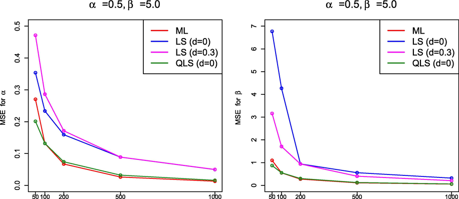
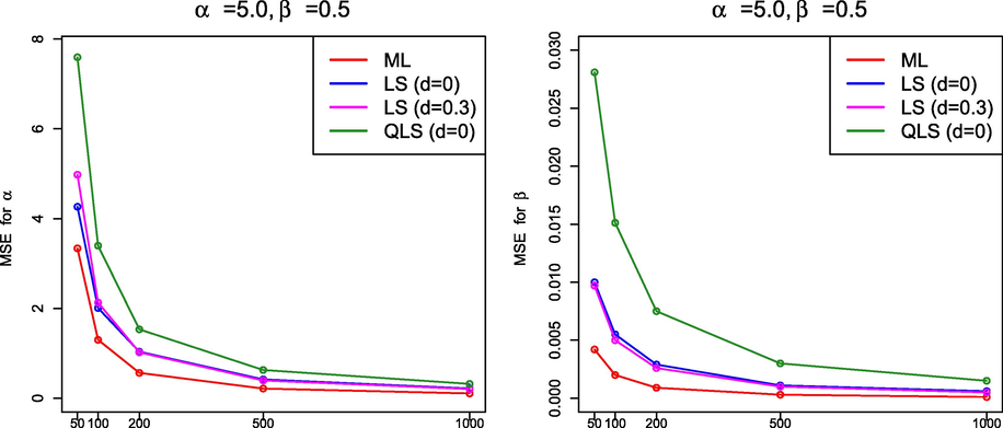
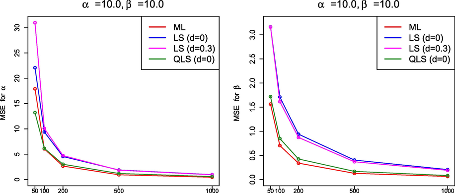
3.3 Simulation findings
From the simulation results in Sections 3.1.1 and 3.2.4, it must be highlighted that, in general, the performance of ML was better than that of the methods based on least squares because the ML method produced estimates with smaller MSE. It is interesting to note that the QLS method also provided good estimates if
but, as far as we have been able to determine, the QLS method did not improve the results obtained by ML. Figs. 7–10 display graphically the behavior of the MSE for the estimation methods under comparison for the values of
and n in Table 1 and Tables 3–5.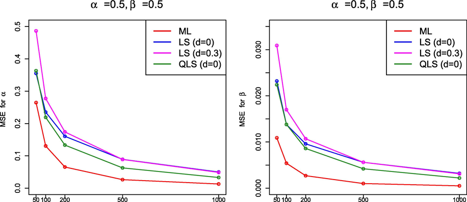
MSE(
) –left– and MSE(
) –right– for
and
.
MSE(
) –left– and MSE(
) –right– for
and
.
MSE(
) –left– and MSE(
) –right– for
and
.
MSE(
) –left– and MSE(
) –right– for
and
.
4 Data analysis
In this section, two real data sets are considered to illustrate that the LSG distribution may be an alternative to other two-parameter models with bounded support.
4.1 Data set 1: Antimicrobial resistance
The first data set is available in the report (European Centre for Disease Prevention and Control, 2013, pp. 178) from of the European Centre for Disease Prevention and Control, which is the main EU surveillance system for antimicrobial (antibiotic) resistance. The data represent the annual percentage of antimicrobial resistant isolates in Portugal in 2012. The (sorted) values are the following: 1, 1, 3, 5, 8, 12, 14, 15, 15, 16, 19, 20, 20, 23, 26, 30, 32, 36, 39, 43, 54, 58, 59, 94.
The LSG law was fitted to the above data (divided by 100) and the ML estimates were
and
. The theoretical cumulative probabilities of the LSG model fit the empirical ones fairly well since the correlation coefficient between them is 0.9927. In order to evaluate the goodness of fit, the following tests were applied: Cramér von Mises statistic
, Watson statistic
, Anderson–Darling statistic
, Kolmogorov–Smirnov statistics
and D, and Kuiper statistic V (see D’Agostino and Stephens, 1986, Chapter 4 for details). To get the corresponding p-values a parametric bootstrap was applied by generating 10,000 bootstrap samples (see Babu and Rao, 2004). The results are shown in Table 6.
D
V
p-value
0.7763
0.7561
0.8503
0.9693
0.4030
0.6499
0.8228
The LSG fitting was compared to the ones provided by other two-parameter laws used to model data in the unit interval, specifically the distributions beta, Kumaraswamy, Log–Lindley (with the reparametrization given in Jodrá and Jiménez-Gamero, 2016), transformed Leipnik and standard two-sided power. The aforesaid models were compared through the Akaike information criterion (AIC) and the Bayesian information criterion (BIC), namely,
and
, where r is the number of parameters, L denotes the maximized value of the likelihood function and n is the sample size. As it is well-known, the model with lower values of AIC and/or BIC is preferred. Table 7 reports the corresponding results and Fig. 11 shows the empirical cdf together with the fitted distributions. The LSG model provided a suitable fit with the smallest AIC and BIC values.
Distributions with support
ML estimates
AIC
BIC
LSG(
)
8.41
Beta(
)
7.52
Kumaraswamy(
)
7.56
Log–Lindley(
)
7.87
Transformed Leipnik(
)
7.80
Two-sided power(
)
7.68
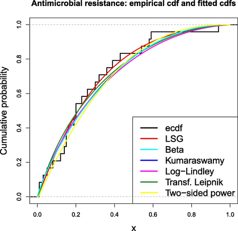
Empirical cdf and fitted cdfs for the antimicrobial resistance data.
4.2 Data set 2: French speakers
The second data set corresponds to percentages of French speakers in 88 countries in 20141. The (sorted) values are the following: 0.1, 0.1, 0.3, 0.4, 0.7, 0.7, 0.8, 0.8, 1, 1, 1, 1, 1, 2, 2, 2, 2, 2, 2, 3, 3, 3, 3, 3, 3, 3, 4, 4, 4, 6, 6, 6, 7, 7, 8, 8, 9, 10, 10, 10, 11, 11, 11, 11, 11, 12, 13, 13, 13, 13, 14, 15, 15, 16, 17, 20, 20, 21, 22, 23, 24, 25, 29, 29, 29, 29, 31, 31, 33, 34, 35, 38, 39, 40, 42, 47, 50, 53, 54, 58, 61, 66, 70, 72, 73, 79, 96, 97.
The LSG distribution was fitted to the data set (divided by 100) and the ML estimates were
and
. The correlation coefficient between the theoretical cumulative probabilities of the LSG model and the empirical ones is 0.9967. As in Section 4.1, the same goodness-of-fit tests were applied and the p-values are shown in Table 8.
D
V
p-value
0.5574
0.5911
0.2744
0.1329
0.8670
0.2363
0.4294
The LSG fitting was compared to the ones provided by the distributions beta, Kumaraswamy, Log–Lindley, transformed Leipnik and standard two-sided power. Table 9 shows the results and the LSG model yielded the smallest AIC and BIC values. Fig. 12 also shows the empirical cdf together with the fitted distributions. Overall, it can be concluded that the LSG model provided a good fit.
Distributions with support
ML estimates
AIC
BIC
LSG(
)
57.69
Beta(
)
54.07
Kumaraswamy(
)
54.89
Log–Lindley(
)
Transformed Leipnik(
)
56.36
Two-sided power(
)
39.85
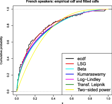
Empirical cdf and fitted cdfs for the French speakers data.
5 Conclusions
A two-parameter probability distribution defined on (0,1) is derived from the shifted Gompertz law. The proposed model also arises as the probability distribution of the minimum of a shifted Poisson random number of independent random variables having a common power function distribution. The new family of distributions has tractable properties. Analytical expressions are provided for the moments, quantile function and moments of the order statistics. The limit behavior of the extreme order statistics is also established. The parameters can be easily estimated by the method of maximum likelihood, which provided better results than other procedures based on least squares.
Acknowledgements
The author thanks the anonymous referees for their constructive comments, which led to a substantial improvement of the paper. Research in this paper has been partially funded by Diputación General de Aragón –Grupo E24-17R– and ERDF funds.
References
- A First Course in Order Statistics. New York: Wiley & Sons Inc; 1992.
- Analysis for the linear failure-rate life-testing distribution. Technometrics. 1974;16:551-559.
- [Google Scholar]
- Balakrishnan N., Rao C.R., eds. Order Statistics: Theory and Methods, Handbook of Statistics. Vol volume 16. Amsterdam: Elsevier; 1998.
- Probability plotting methods and order statistics. J. Roy. Statist. Soc. Ser. C Appl. Statist.. 1975;24:95-108.
- [Google Scholar]
- Modelling the diffusion of new durable goods: word-of-mouth effect versus consumer heterogeneity. In: Laurent G., Lilien G.L., Pras B., eds. Research Traditions in Marketing. Boston: Kluwer; 1994. p. :201-229.
- [Google Scholar]
- The impact of heterogeneity and ill–conditioning on diffusion model parameter estimates. Market. Sci.. 2002;21(2):209-220.
- [Google Scholar]
- Mathematical Statistics, Basic Ideas and Selected Topics Vol vol. 1. (2nd edition). New Jersey: Prentice Hall; 2001.
- The exponentiated Kumaraswamy-power function distribution. Hacet. J. Math. Stat.. 2017;46(2):277-292.
- [Google Scholar]
- Condino, F., Domma, F., A new distribution function with bounded support: the reflected generalized Topp-Leone power series distribution, Metron 75 (1) 51–68, 2017.
- The Kumaraswamy Weibull distribution with application to failure data. J. Franklin Inst.. 2010;347(8):1399-1429.
- [Google Scholar]
- D’Agostino R.B., Stephens M.A., eds. Goodness-of-Fit-Techniques. New York: Marcel Dekker; 1986.
- Antimicrobial resistance surveillance in Europe 2012, Annual Report of the European Antimicrobial Resistance Surveillance Network (EARS-Net). Stockholm: ECDC; 2013. URL https://ecdc.europa.eu
- Monte Carlo: Concepts, Algorithms and Applications, Springer Series in Operations Research. New York: Springer-Verlag; 1996.
- The Log-Lindley distribution as an alternative to the beta regression model with applications in insurance. Insur. Math. Econ.. 2014;54:49-57.
- [Google Scholar]
- Estimation of parameters of the shifted Gompertz distribution using least squares, maximum likelihood and moments methods. J. Comput. Appl. Math.. 2014;255:867-877.
- [Google Scholar]
- A note on the moments and computer generation of the shifted Gompertz distribution. Commun. Stat.-Theory Methods. 2009;38(1–2):75-89.
- [Google Scholar]
- Kumaraswamy’s distribution: a beta-type distribution with some tractability advantages. Stat. Methodol.. 2009;6(1):70-81.
- [Google Scholar]
- The Theory of Dispersion Models. London: Chapman & Hall; 1997.
- Nonlinear least squares estimation of the shifted Gompertz distribution. Eur. J. Pure Appl. Math.. 2017;10(2):157-166.
- [Google Scholar]
- A new generalized two-sided class of distributions with an emphasis on two-sided generalized normal distribution. Comm. Statist. Simul. Comput.. 2017;46(2):1441-1460.
- [Google Scholar]
- Beyond beta. Other continuous families of distributions with bounded support and applications. Hackensack, NJ: World Scientific Publishing Co., Pte. Ltd.; 2004.
- Generalized probability density function for double-bounded random processes. J. Hydrol.. 1980;46(1–2):79-88.
- [Google Scholar]
- Theory of Point Estimation. In: Springer Texts in Statistics (second ed.). New York: Springer-Verlag; 1998.
- [Google Scholar]
- Some generalized functions for the size distribution of income. Econometrica. 1984;52(3):647-663.
- [Google Scholar]
- Incomplete gamma and related functions. In: Olver F.W.F., Lozier D.W., Boisvert R.F., Clark C.W., eds. NIST Handbook of Mathematical Functions, National Institute of Standards and Technology. Washington, DC: Cambridge University Press, Cambridge; 2010. p. :173-192.
- [Google Scholar]
- The Kumaraswamy generalized gamma distribution with application in survival analysis. Stat. Methodol.. 2011;8:411-433.
- [Google Scholar]
- R: A language and environment for statistical computing. Vienna, Austria: R Foundation for Statistical Computing; 2018. URL http://www.R-project.org/
- Stochastic Orders. New York: Springer-Verlag; 2007.
- The standard two-sided power distribution and its properties: with applications in financial engineering. Amer. Statist.. 2002;56(2):90-99.
- [Google Scholar]


