A new numerical scheme for solving pantograph type nonlinear fractional integro-differential equations

H. Jafari; N.A. Tuan; R.M. Ganji

doi:10.1016/j.jksus.2020.08.029

View/Download PDF

Buy Reprints

PDF

Translate this page into:

Original article

01 2020

:33;

101185

doi:

10.1016/j.jksus.2020.08.029

A new numerical scheme for solving pantograph type nonlinear fractional integro-differential equations

H. Jafari^{^a,^b,^c}, N.A. Tuan^{^d,⁎}, R.M. Ganji^{^a,^b}

a Department of Mathematic, University of Mazandaran, Babolsar, Iran

b Department of Mathematical Sciences, University of South Africa, UNISA0003, South Africa

c Department of Medical Research, China Medical University Hospital, China Medical University, Taichung 110122, Taiwan

d Division of Applied Mathematics, Thu Dau Mot University, Binh Duong Province, Viet Nam

⁎Corresponding author. nguyenanhtuan@tdmu.edu.vn (N.A. Tuan)

Received: 2020-6-5, Accepted: 2020-8-22,

Disclaimer:
This article was originally published by Elsevier and was migrated to Scientific Scholar after the change of Publisher.

Abstract

In this work, a general class of pantograph type nonlinear fractional integro-differential equations (PT-FIDEs) with non-singular and non-local kernel is considered. A numerical scheme based on the orthogonal basis functions including the shifted Legendre polynomials (SLPs) is proposed. First, we expand the unknown function and its derivatives in terms of the SLPs with unknown coefficients. Then, we present several theorems based on the SLPs for the help to achieve the approximate solution of the problem under study. Finally, by utilizing these theorems together with the collocation points, the main problem is transformed to a system of linear or nonlinear algebraic equations, which can be simply solved. An investigation for error estimate is discussed. The accuracy and efficiency of the proposed scheme are reported by four illustrative examples.

Keywords

Non-local and non-singular kernel

Volterra nonlinear fractional integro-differential equations

Atangana–Baleanu operator

The shifted Legendre polynomials

Approximation solution

34A08

65M70

11B68

1 Introduction

Fractional calculus is an extension of the classical one which deal with derivatives and integrals of arbitrary real or complex order (Atangana and Hammouch, 2019; Baleanu et al., 2012; Podlubny, 1999; Srivastava et al., 2021; Yang et al., 2020 ). Fractional derivatives have been widely applied to describing various problems in different fields of applied science. These derivatives are useful in rheology as crucial features of cell rheological behavior (Djordjevic et al., 2003). Recently, the dynamics of coronavirus (2019-nCov) have modeled by with fractional derivative in Khan and Atangana (2020). Since in definition of the most important fractional operators such as Riemann–Liouville (RL) and Caputo exists a kernel of type local and sinqular, it is difficult or impossible to describe many non-local dynamics systems. Hence several definitions for fractional integral and derivative operators have been introduced such as Caputo–Fabrizio (CF) (Caputo and Fabrizio, 2015; Losada and Nieto, 2015), Atangana–Baleanu (AB) (Atangana and Baleanu, 2016) and Yang–Abdel–Aty–Cattani (YAAC) (Yang et al., 2019) operators. The most important advantage of these operators is the existence of the non-local and non-sinqular kernel which introduced to describe complex physical problems (Algahtani, 2016; Djida et al., 2017).

In this work, we consider a class of PT-FIDEs of the form

(1)

^{ABC} D_{t}^{α} z (t) = λ F (t, z (t), z (qt), I_{t} z (t), I_{qt} z (t)), t \in [0, T], 0 < q < 1, 0 < α ⩽ 1,

with

(2)

\begin{matrix} I_{t} z (t) = \int_{0}^{t} K_{1} (t, τ) ϕ_{1} (τ, z (τ)) d τ, \\ I_{qt} z (t) = \int_{0}^{qt} K_{2} (t, τ) ϕ_{2} (τ, z (τ)) d τ, \end{matrix}

and the initial condition

(3)

z (0) = z_{0},

where

λ

and

z_{0}

are real constants,

K_{1}, K_{2}, ϕ_{1}

and

ϕ_{2}

are given functions,

z (t)

is a solution to be determined in

[0, T]

^{ABC} D_{t}^{α}

denotes the AB derivative in the Caputo sense. This new fractional derivative is introduced by Atangana and Baleanu which has non-singular kernel. In definition of this operator, there exists a kernel that is included a Mittag–Leffler (ML) function which is non-local and non-singular. Many properties of this operator are investigated in Atangana and Kocab (2016). The special cases of the Eq. (1) have been solved in Muroya et al. (2003), Rahimkhani et al. (2017), Zhao et al. (2017), Nemati et al. (2018).

Volterra nonlinear fractional integro-differential equations (V-NFIDEs) appear widely in many fields of science. The class of PV-IDEs is one of the most important classes of V-FIDEs. Many researchers have presented several numerical techniques for solving these equations (Muroya et al., 2003; Rahimkhani et al., 2017; Zhao et al., 2017 ).

Orthogonal basis functions have been generally used to achieve approximate solution for many problems in various fields of science. Approximation of the solution using these functions is known as a useful tool in solving many classes of equations, numerically, e.g., differential equations (Jafari et al., 2011; Mishra et al., 2016; Sabermahani et al., 2018; Sabermahani et al., 2020; Singh and Srivastava, 2019; Srivastava et al., 2019 ), partial differential equations (Ait Touchent et al., 2018; Deiveegan et al., 2019; Ganji et al., 2019; Yang et al., 2018; Yang and Tenreiro Machado, 2017; Ziane et al., 2019 ) and integro-differential equations (Ganji and Jafari, 2020; Ganji and Jafari, 2019; Nemati et al., 2018; Sedaghat et al., 2014; Nieto and Samet, 2017; Jothimani et al., 2019 ) of various orders (fixed, fractional or variable order).

The outline of this work is as follows. A brief review of definitions of RL and AB operators and their important properties are presented in Section 2. Section 3 the SLPs with their properties are reviewed. We proposed a numerical scheme for solving problem (1) under the initial condition given by (3) in section (4). In section (5), we discussed about error bound of the proposed scheme. Some illustrative examples are solved in Section 6. In the last section, we conclude the paper.

2 RL and AB operators and their properties

In this section, we first recall many special functions and then bring definitions of (RL and AB)- integral and derivative operators with their properties which will be used further.

Definition 1

Definition 1 See Podlubny (1999)

The Beta and Mittag–Leffler functions are defined, respectively, by $\begin{matrix} (The Beta function) B (μ, ν) = \int_{0}^{1} τ^{μ - 1} {(1 - τ)}^{ν - 1} d τ, Re (μ) & Re (ν) > 0, \\ (One parameter ML function) E_{α} (t) = \sum_{i = 0}^{\infty} \frac{t^{i}}{Γ (α i + 1)}, \\ (Two parameters ML function) E_{α, β} (t) = \sum_{i = 0}^{\infty} \frac{t^{i}}{Γ (α i + β)} . \end{matrix}$

Definition 2

Definition 2 See Podlubny (1999)

The $α$ order RL-integral is given by $^{RL} I_{t}^{α} z (t) = \frac{1}{Γ (α)} \int_{0}^{t} {(t - τ)}^{α - 1} z (τ) d τ .$

The RL-integral of order $α$ satisfies the following property $^{RL} I_{t}^{α} t^{ζ} = \frac{Γ (1 + ζ)}{Γ (α + ζ + 1)} t^{α + ζ}, ζ ⩾ 0 .$

Definition 3

Definition 3 See Atangana and Baleanu (2016), Yang (2019)

Let $0 < α ⩽ 1, z \in H^{1} (0, 1)$ and $ℵ (α)$ be a normalization function such that $ℵ (0) = ℵ (1) = 1$ and for $0 < α < 1, ℵ (α) = 1 - α + \frac{α}{Γ (α)}$ . Then

(1) The ABC-derivative is defined as follows
(4)
$^{ABC} D_{t}^{α} z (t) = \{\begin{matrix} \frac{AB (α)}{1 - α} \int_{0}^{t} E_{α} (- \frac{α}{1 - α} {(t - τ)}^{α}) z' (τ) d τ, \\ z' (t) & α = 1 . \end{matrix}$
(2) The AB-integral is given by
(5)
$^{AB} I_{t}^{α} z (t) = \frac{1 - α}{ℵ (α)} z (t) + \frac{α}{ℵ (α) Γ (α)} \int_{0}^{t} {(t - τ)}^{α - 1} z (τ) d τ .$

Let $υ_{α} = \frac{1 - α}{ℵ (α)}$ and $ω_{α} = \frac{1}{ℵ (α) Γ (α)}$ , then we can rewrite (5) by

(6)

^{AB} I_{t}^{α} z (t) = υ_{α} z (t) + ω_{α} Γ (α + 1)^{RL} I_{t}^{α} z (t) .

It is easy to report that the AB operators satisfy the following properties (Atangana and Baleanu, 2016; Ganji and Jafari, 2020; Ganji et al., 2020 ) $\begin{matrix} ^{ABC} D_{t}^{α} C = 0, C \in R, \\ ^{ABC} D_{t}^{α} t^{β} = \frac{ℵ (α) β! t^{β}}{1 - α} E_{α, 1 + β} (- \frac{α}{1 - α} t^{α}), β ⩾ 0, \\ ^{AB} I_{t}^{α} C = C (υ_{α} + ω_{α} t^{α}), C \in R, \\ ^{AB} I_{t}^{α} t^{β} = t^{β} (υ_{α} + ω_{α} (α + 1 + β) B (1 + β, 1 + α) t^{α}), \\ ^{AB} I_{t}^{α} (^{ABC} D_{t}^{α} z (t)) = z (t) - z (0) . \end{matrix}$

Theorem 1

Theorem 1 See Tajadodi (2020)

Let $0 < α ⩽ 1$ . Then, we can rewrite the AB-derivative by $^{ABC} D_{t}^{α} z (t) = \frac{AB (α)}{1 - α} \sum_{r = 0}^{\infty} {(\frac{- α}{1 - α})}^{r}^{RL} I_{t}^{r α + 1} z' (t) .$

3 The SLPs and their properties

Now, firstly we express some basic properties of the SLPs. After that we explain to approximate a function with SLPs and obtaining OM based on SLPs.

3.1

3.1 The SLPs

The explanation of the SLPs on $[0, T]$ is

(7)

L_{i}^{*} (t) = L_{i} (\frac{2}{T} t - 1), i = 0, 1, 2, \dots,

where

L_{i} (t)

is the well-known Legendre polynomial (LP) of degree i. The recursive formula of LP on

[- 1, 1]

given by

L_{i + 1} (t) = \frac{1 + 2 i}{1 + i} t L_{i} (t) - \frac{i}{1 + i} L_{i - 1} (t), i = 1, 2, 3, \dots,

where

L_{0} (t) = 1

and

L_{1} (t) = t

The SLPs $L_{i}^{*} (t)$ given in (7), could be written the following analytic form

(8)

L_{i}^{*} (t) = \sum_{s = 0}^{i} a_{i, s} t^{s},

where

(9)

a_{i, s} = \frac{{(- 1)}^{i + s} (i + s)!}{(i - s)! {(s!)}^{2} T^{s}} .

For the SLPs, the orthogonality condition is as follows $\int_{0}^{T} L_{i}^{*} (t) L_{s}^{*} (t) dt = \{\begin{matrix} \frac{T}{1 + 2 i}, & i = s, \\ 0, & i \neq s . \end{matrix}$

For two arbitrary functions $z_{1}, z_{2}$ in $L^{2} (0, T)$ , the inner product and norm are defined, respectively, by $\begin{matrix} 〈 z_{1} (t), z_{2} (t) 〉 = \int_{0}^{T} z_{1} (t) z_{2} (t) dt, \\ ∥ z_{1} (t) ∥_{L^{2} (0, T)} = 〈 z_{1} (t), z_{1} (t) 〉^{\frac{1}{2}} = {(\int_{0}^{T} ∣ z_{1} (t) ∣^{2} dt)}^{\frac{1}{2}} . \end{matrix}$

3.2

3.2 Approximation of a function

Assume that we can expand $z (t) \in L^{2} (0, T)$ in terms of the SLPs as

(10)

z (t) = \sum_{i = 0}^{\infty} z_{i} L_{i}^{*} (t),

where

z_{i} = \frac{1 + 2 i}{T} \int_{0}^{T} z (t) L_{i}^{*} (t) dt .

We can present z by using a truncated series as

(11)

z (t) ≃ z_{M} (t) = \sum_{i = 0}^{M} z_{i} L_{i}^{*} (t) = Z^{T} L (t),

where

Z = {[z_{0}, z_{1}, \dots, z_{M}]}^{T}

and

(12)

L (t) = {[L_{0}^{*} (t), L_{1}^{*} (t), \dots, L_{M}^{*} (t)]}^{T} .

Also, we can approximate the function $z (t, τ) \in L^{2} ((0, T) \times (0, T))$ in terms of the SLPs by $z (t, τ) ≃ L^{T} (t) Z L (τ),$ where $Z = [z_{i, j}]$ is an $(M + 1) \times (M + 1)$ matrix which $z_{i, j}, i, j = 0, 1, \dots, M$ are given by $z_{i, j} = \frac{〈 〈 z (t, τ), L_{i}^{*} (t) 〉, L_{j}^{*} (τ) 〉}{∥ L_{i}^{*} (t) ∥_{2}^{2} ∥ L_{j}^{*} (τ) ∥_{2}^{2}}, i, j = 0, 1, \dots, M .$

Lemma 1

Suppose $0 < q < 1$ and $L (t)$ given by (12). Then $L (qt) ≃ HL (t),$ where $H$ is given by $H = [\begin{matrix} σ_{0, 0, 0} & σ_{0, 1, 0} & \dots & σ_{0, M, 0} \\ \sum_{s = 0}^{1} σ_{1, 0, s} & \sum_{s = 0}^{1} σ_{1, 1, s} & \dots & \sum_{s = 0}^{1} σ_{1, M, s} \\ ⋮ & ⋮ & \dots & ⋮ \\ \sum_{s = 0}^{M} σ_{M, 0, s} & \sum_{s = 0}^{M} σ_{M, 1, s} & \dots & \sum_{s = 0}^{M} σ_{M, M, s} \end{matrix}],$ with $σ_{i, k, s} = a_{i, s} h_{s, k} q^{s} .$

Proof

By substituting $t = qt$ into (8), we get

(13)

L_{i}^{*} (qt) = \sum_{s = 0}^{i} a_{i, s} q^{s} t^{s} i = 0, 1, \dots, M .

Now, we approximate the function $t^{s}$ in terms of the SLPs by

(14)

t^{s} ≃ \sum_{k = 0}^{M} h_{s, k} L_{k}^{*} (t) .

Now for $i = 0$ to $i = M$ , By substituting (14) into (13), leads $L_{i}^{*} (qt) ≃ \sum_{s = 0}^{i} a_{i, s} q^{s} (\sum_{k = 0}^{M} h_{s, k} L_{k}^{*} (t)) = \sum_{k = 0}^{M} (\sum_{s = 0}^{i} a_{i, s} h_{s, k} q^{s}) L_{k}^{*} (t) = \sum_{k = 0}^{M} (\sum_{s = 0}^{i} σ_{i, k, s}) L_{k}^{*} (t),$ which completes the proof.

Lemma 2

Lemma 2 See Ganji et al. (2020)

The operational matrix (OM) of the product and integration of the vector $L (t)$ given by (12) can be approximated, respectively, as $\begin{matrix} L (t) L^{T} (t) Z ≃ \hat{Z} L (t), \\ \int_{0}^{t} L (τ) d τ ≃ P L (t), \end{matrix}$ where $\hat{Z}$ and $P$ are given in Ganji et al. (2020).

Theorem 2

Suppose $L (t)$ given by (12). Then $\int_{0}^{qt} L (τ) d τ ≃ P^{*} L (t),$ where $P^{*}$ is given by $P^{*} = [\begin{matrix} ς_{0, 0, 0} & ς_{0, 1, 0} & \dots & ς_{0, M, 0} \\ \sum_{s = 0}^{1} ς_{1, 0, s} & \sum_{s = 0}^{1} ς_{1, 1, s} & \dots & \sum_{s = 0}^{1} ς_{1, M, s} \\ ⋮ & ⋮ & \dots & ⋮ \\ \sum_{s = 0}^{M} ς_{M, 0, s} & \sum_{s = 0}^{M} ς_{M, 1, s} & \dots & \sum_{s = 0}^{M} ς_{M, M, s} \end{matrix}],$ with $ς_{i, k, s} = \frac{a_{i, s} d_{s, k} q^{s + 1}}{s + 1} .$

Proof

By (12), for $i = 0, 1, \dots, M$ , we have

(15)

\int_{0}^{qt} L_{i}^{*} (τ) d τ = \int_{0}^{qt} (\sum_{s = 0}^{i} a_{i, s} τ^{s}) d τ = \sum_{s = 0}^{i} a_{i, s} (\int_{0}^{qt} τ^{s} d τ) = \sum_{s = 0}^{i} \frac{a_{i, s} q^{s + 1}}{s + 1} t^{s + 1},

We expand $t^{s + 1}$ in the above equation by using the SLPs. It gives

(16)

t^{s + 1} ≃ \sum_{k = 0}^{M} d_{s, k} L_{k}^{*} (t) .

By putting (16) into (15), we get $\int_{0}^{qt} L_{i}^{*} (τ) d τ ≃ \sum_{s = 0}^{i} \frac{a_{i, s} q^{s + 1}}{s + 1} (\sum_{k = 0}^{M} d_{s, k} L_{k}^{*} (t)) = \sum_{k = 0}^{M} (\sum_{s = 0}^{i} \frac{a_{i, s} d_{s, k} q^{s + 1}}{s + 1}) L_{k}^{*} (t) = \sum_{k = 0}^{M} (\sum_{s = 0}^{i} ς_{i, k, s}) L_{k}^{*} (t),$ now the proof is completed.

Theorem 3

Suppose $0 < α ⩽ 1$ . The $α$ order AB-integral of a vector $L (t)$ given in (12) might be approximated by $^{AB} I_{t}^{α} L (t) ≃ I^{α} L (t),$ where $I^{α} = υ_{α} I + ω_{α} Γ (α + 1) F^{α}$ is called the OM of the AB-integral based on the SLPs and I is an $(M + 1) \times (M + 1)$ identity matrix. Also, $F^{α}$ is called the OM of RL-integral based on the SLPs which is given by $F^{α} = [\begin{matrix} ρ_{0, 0, 0} & ρ_{0, 1, 0} & \dots & ρ_{0, M, 0} \\ \sum_{s = 0}^{1} ρ_{1, 0, s} & \sum_{s = 0}^{1} ρ_{1, 1, s} & \dots & \sum_{s = 0}^{1} ρ_{1, M, s} \\ ⋮ & ⋮ & \dots & ⋮ \\ \sum_{s = 0}^{M} ρ_{M, 0, s} & \sum_{s = 0}^{M} ρ_{M, 1, s} & \dots & \sum_{s = 0}^{M} ρ_{M, M, s} \end{matrix}],$ with $ρ_{i, k, s} = \frac{Γ (s + 1) a_{i, s} e_{s, k}}{Γ (s + α + 1)} .$

Proof

By applying the AB-integral operator on the vector $L (t)$ yields

(17)

^{AB} I_{t}^{α} L (t) = υ_{α} L (t) + ω_{α} Γ (α + 1)^{RL} I_{t}^{α} L (t) .

Now, we must obtain the OM of RL-integral of order $α$ . To do this, we apply the LR-integral operator, $^{RL} I_{t}^{α}$ , on $L_{i}^{*} (t), i = 0, 1, \dots, M$ as $^{RL} I_{t}^{α} L_{i}^{*} (t) =^{RL} I_{t}^{α} (\sum_{s = 0}^{i} a_{i, s} t^{s}) = \sum_{s = 0}^{i} a_{i, s} (^{RL} I_{t}^{α} t^{s}) = \sum_{s = 0}^{i} \frac{Γ (s + 1) a_{i, s}}{Γ (s + α + 1)} t^{s + α} .$

By approximating the function $t^{s + α}$ in terms of the SLPs, we get

(18)

t^{s + α} ≃ \sum_{k = 0}^{M} e_{s, k} L_{k}^{*} (t) .

In view of (18) and for $i = 0, 1, \dots, M$ , we get $\begin{matrix} ^{RL} I_{t}^{α} L_{i}^{*} (t) ≃ \sum_{s = 0}^{i} \frac{Γ (s + 1) a_{i, s}}{Γ (s + α + 1)} (\sum_{k = 0}^{M} e_{s, k} L_{k}^{*} (t)) = \sum_{k = 0}^{M} (\sum_{s = 0}^{i} \frac{Γ (s + 1) a_{i, s} e_{s, k}}{Γ (s + α + 1)}) L_{k}^{*} (t) \\ = \sum_{k = 0}^{M} (\sum_{s = 0}^{i} ρ_{i, k, s}) L_{k}^{*} (t) . \end{matrix}$

Therefore, for $i = 0, 1, \dots, M$ , we can write

(19)

^{RL} I_{t}^{α} L (t) = F^{α} L (t),

where

F^{α} = [\begin{matrix} ρ_{0, 0, 0} & ρ_{0, 1, 0} & \dots & ρ_{0, M, 0} \\ \sum_{s = 0}^{1} ρ_{1, 0, s} & \sum_{s = 0}^{1} ρ_{1, 1, s} & \dots & \sum_{s = 0}^{1} ρ_{1, M, s} \\ ⋮ & ⋮ & \dots & ⋮ \\ \sum_{s = 0}^{M} ρ_{M, 0, s} & \sum_{s = 0}^{M} ρ_{M, 1, s} & \dots & \sum_{s = 0}^{M} ρ_{M, M, s} \end{matrix}],

with

ρ_{i, k, s} = \frac{Γ (s + 1) a_{i, s} e_{s, k}}{Γ (s + α + 1)} .

By substituting (19) into (17), the proof completes.

4 Numerical scheme

The purpose of this section is to present a numerical scheme for solving Eq. (1) under the initial condition (3). To this aim, we first approximate the function $^{ABC} D_{t}^{α} z (t)$ in terms of the SLPs as

(20)

^{ABC} D_{t}^{α} z (t) ≃ Z^{T} L (t) .

First we apply the $α$ order AB-integral on the both sides of (20) and use the initial condition, we have

(21)

z (t) ≃ Z^{T} I^{α} L (t) + z_{0} .

By approximating $z_{0} ≃ B^{T} L (t)$ , (21) is rewritten as

(22)

z (t) ≃ YL (t),

where

Y = Z^{T} I^{α} + B^{T}

. By putting

t = qt

in (22) yields

(23)

z (qt) ≃ YL (qt) .

By employing Lemma 1, (23) is approximated as

(24)

z (qt) ≃ YHL (t) .

For approximating the Volterra parts of Eq. (1), we expand $K_{1}, K_{2}, ϕ_{1}$ and $ϕ_{2}$ using the SLPs as

(25)

\begin{matrix} K_{1} (t, τ) ≃ L^{T} (t) K_{1} L (τ), \\ K_{2} (t, τ) ≃ L^{T} (t) K_{2} L (τ), \\ ϕ_{1} (t, z (t)) ≃ C^{T} L (τ), \\ ϕ_{2} (t, z (t)) ≃ D^{T} L (τ) . \end{matrix}

By utilizing (25), Lemma 2, Theorem 2, and in a similar way (Ganji et al., 2020), we obtain

(26)

\begin{matrix} I_{t} z (t) & ≃ \int_{0}^{t} (L^{T} (t) K_{1} L (τ)) (L^{T} (τ) C) d τ = L^{T} (t) K_{1} \hat{C} \int_{0}^{t} L (τ) d τ = L^{T} (t) K_{1} \hat{C} PL (t), \\ I_{qt} z (t) & ≃ \int_{0}^{qt} (L^{T} (t) K_{2} L (τ)) (L^{T} (τ) D) d τ = L^{T} (t) K_{2} \hat{D} \int_{0}^{qt} L (τ) d τ = L^{T} (t) K_{2} \hat{D} P^{*} L (t) . \end{matrix}

Substituting (20), (22), (24) and (26) into Eq. (1), leads

(27)

Z^{T} L (t) = λ F (t, YL (t), YHL (t), L^{T} (t) K_{1} \hat{C} PL (t), L^{T} (t) K_{2} \hat{D} P^{*} L (t)) .

Also, by substituting (20) into (25) yields

(28)

\begin{matrix} ϕ_{1} (t, YL (t)) ≃ C^{T} L (t), \\ ϕ_{2} (t, YL (t)) ≃ D^{T} L (t) . \end{matrix}

Finally, by substituting the collocation points $\frac{k}{M + 2} T, k = 1, \dots, M + 1$ into Eqs. (27) and (28), a system of $3 (M + 1)$ nonlinear equations of the vectors of $Z, C$ and $D$ is formed. By solving this system, the unknown parameters of the vectors of $Z, C$ and $D$ are obtained. Finally the approximate solution can be computed by (22).

5 Error estimation

This section deals an estimate for the error of the numerical solution of Eq. (1) with initial condition (3) obtained by the proposed scheme in Section 4.

It is well known in the interval $(a, b)$ , the Sobolev norm of integer order $μ ⩾ 0$ , is defined by $‖ z ‖_{H^{μ} (a, b)} = {(\sum_{k = 0}^{μ} ‖ z^{(k)} ‖_{L^{2} (a, b)})}^{\frac{1}{2}},$ where $z^{(k)}$ denotes the kth derivative of z and $H^{μ} (a, b)$ is a Sobolev space.

Lemma 3

Lemma 3 See Canuto et al. (2006)

Let $μ ⩾ 0$ and $z \in H^{m} (- 1, 1)$ . Suppose $P_{M} (z) = \sum_{i = 0}^{M} z_{i} L_{i} (t)$ be the truncated Legendre series of z. Then, $‖ z - P_{M} (z) ‖_{L^{2} (- 1, 1)} ⩽ {CM}^{- μ} | z |_{H^{μ; M} (- 1, 1)},$ where $| z |_{H^{μ; M} (- 1, 1)} = {(\sum_{k = \min {1 + M, μ}}^{μ} ‖ z^{(k)} ‖_{L^{2} (- 1, 1)}^{2})}^{\frac{1}{2}},$ and C is a positive constant and does not depend to z and integer M.

Lemma 4

Lemma 4 See Ganji et al. (2020)

Let $z : (0, T) ⟶ R$ be a function in $H^{μ} (0, T)$ . Suppose that function $\bar{z} : (- 1, 1) ⟶ R$ is given by $\bar{z} (t) = z (\frac{T}{2} (t + 1))$ for all $t \in (- 1, 1)$ . Then, for $0 ⩽ k ⩽ μ$ $‖ {\bar{z}}^{(k)} ‖_{L^{2} (- 1, 1)} = {(\frac{2}{T})}^{\frac{1}{2} - k} ‖ z^{(k)} ‖_{L^{2} (0, T)} .$

Theorem 4

Suppose $μ ⩾ 0$ and $z \in H^{μ} (0, T)$ . Let $z_{M} (t) = \sum_{i = 0}^{M} z_{i} L_{i}^{*} (t)$ is the obtained approximate solution by the given scheme in Section 4. Then, $‖ z - z_{M} ‖_{L^{2} (0, T)} ⩽ {CM}^{- μ} | z |_{H^{μ; M; 0} (0, T)},$ and $‖ z^{(i)} - z_{M}^{(i)} ‖_{L^{2} (0, T)} ⩽ {CM}^{- μ} | z |_{H^{μ; M; i} (0, T)},$ where $| z |_{H^{μ; M; r} (0, T)} = {(\sum_{k = \min {1 + M, μ}}^{μ} {(\frac{T}{2})}^{2 k} ‖ z^{(k + r)} ‖_{L^{2} (0, T)}^{2})}^{\frac{1}{2}}, r ⩾ 0 .$

Proof

With the help Lemma 4, we obtain $\begin{matrix} ‖ z - z_{M} ‖_{L^{2} (0, T)}^{2} = & \frac{T}{2} ‖ \overline{z} - P_{M} (\overline{z}) ‖_{L^{2} (- 1, 1)}^{2} \\ ⩽ \frac{T}{2} C' M^{- 2 μ} \sum_{k = \min {1 + M, μ}}^{μ} ‖ {\bar{z}}^{(k)} ‖_{L^{2} (- 1, 1)}^{2} \\ = C' M^{- 2 μ} \sum_{k = \min {1 + M, μ}}^{μ} {(\frac{T}{2})}^{2 k} ‖ z^{(k)} ‖_{L^{2} (0, T)}^{2} . \end{matrix}$

By definition $| z |_{H^{μ; M; 0} (0, T)} = {(\sum_{k = \min {1 + M, μ}}^{μ} {(\frac{T}{2})}^{2 k} ‖ z^{(k)} ‖_{L^{2} (0, T)}^{2})}^{\frac{1}{2}},$ the proof completes. By similar way, we obtain $‖ z^{(i)} - z_{M}^{(i)} ‖_{L^{2} (0, T)} ⩽ {CM}^{- μ} | z |_{H^{μ; M; i} (0, T)},$ where $| z |_{H^{μ; M; i} (0, T)} = {(\sum_{k = \min {μ, M + 1}}^{μ} {(\frac{T}{2})}^{2 k} ‖ z^{(k + i)} ‖_{L^{2} (0, T)}^{2})}^{\frac{1}{2}} .$

Theorem 5

Suppose $0 < α ⩽ 1$ and $z \in H^{μ} (0, T)$ satisfies in Theorem 4. Then $‖^{ABC} D_{t}^{α} z -^{ABC} D_{t}^{α} z_{M} ‖_{L^{2} (0, T)} ⩽ \frac{AB (α) T}{1 - α} E_{α, 2} (- \frac{α}{1 - α} T^{α}) {CM}^{- μ} | z |_{H^{μ, M, 1} (0, T)} .$

Proof

By employing Theorems 1 and 4, we get $\begin{matrix} ‖^{ABC} D_{t}^{α} z -^{ABC} D_{t}^{α} z_{M} ‖_{L^{2} (0, T)} = & {‖\frac{AB (α)}{1 - α} \sum_{r = 0}^{\infty} {(\frac{- α}{1 - α})}^{r}^{RL} I_{t}^{r α + 1} (z' - z_{M}')‖}_{L^{2} (0, T)} \\ ⩽ \frac{AB (α)}{1 - α} \sum_{r = 0}^{\infty} {(\frac{- α}{1 - α})}^{r} \frac{T^{r α + 1}}{Γ (r α + 2)} {‖z' - z_{M}'‖}_{L^{2} (0, T)} \\ ⩽ \frac{AB (α) T}{1 - α} E_{α, 2} (- \frac{α}{1 - α} T^{α}) {CM}^{- μ} | z |_{H^{μ, M, 1} (0, T)} . \end{matrix}$

Lemma 5

Suppose $k_{1} = \max_{0 ⩽ t, τ ⩽ T} |K_{1} (t, τ)|, k_{2} = \max_{0 ⩽ t, τ ⩽ T} |K_{2} (t, τ)|$ , and $ϕ_{1}$ and $ϕ_{2}$ satisfy the Lipschitz conditions with the constants $L_{1}$ and $L_{2}$ , respectively. Let $z \in H^{μ} (0, 1)$ satisfies in Theorem 4. Then $\begin{matrix} {‖I_{t} z - I_{t} z_{M}‖}_{L^{2} (0, T)} ⩽ k_{1} L_{1} {TCM}^{- μ} | z |_{H^{μ, M, 0} (0, T)}, \\ {‖I_{t} z - I_{qt} z_{M}‖}_{L^{2} (0, T)} ⩽ k_{2} L_{2} {qTCM}^{- μ} | z |_{H^{μ, M, 0}, (0, T)} . \end{matrix}$

Proof

According to (2) and using Theorem 4, the proof completes.

Theorem 6

Suppose $μ ⩾ 0$ and $z \in H^{μ} (0, T)$ satisfies in Theorems 4, 5 and Lemma 5. Let F satisfies the Lipschitz conditions with the constant L. Then $E_{M}$ , the error bound of the proposed scheme, is bounded as follows $‖ E_{M} ‖_{L^{2} (0, T)} ⩽ {CM}^{- μ} T (\frac{AB (α)}{1 - α} E_{α, 2} (- \frac{α}{1 - α} T^{α}) | z |_{H^{μ, M, 1} (0, T)} + ∣ λ ∣ L (\frac{2}{T} + k_{1} L_{1} + k_{2} L_{2} q) | z |_{H^{μ, M, 0} (0, T)}) .$

Proof

In view of Eq. (1), we get $\begin{matrix} ‖ E_{M} ‖_{L^{2} (0, T)} ⩽ & ‖^{ABC} D_{t}^{α} z -^{ABC} D_{t}^{α} z_{M} - λ F (t, z (t), z (qt), I_{t} z (t), I_{qt} z (t)) \\ {+ λ F (t, z_{M} (t), z_{M} (qt), I_{t} z_{M} (t), I_{qt} z_{M} (t))‖}_{L^{2} (0, T)} \\ ⩽ {‖^{ABC} D_{t}^{α} z -^{ABC} D_{t}^{α} z_{M}‖}_{L^{2} (0, T)} + ∣ λ ∣ L (2 ‖ z - z_{M} ‖_{L^{2} (0, T)} \\ + ‖ I_{t} z - I_{t} z_{M} ‖_{L^{2} (0, T)} + ‖ I_{qt} z - I_{qt} z_{M} ‖_{L^{2} (0, T)}) . \end{matrix}$ By employing Theorems 4, 5 and Lemma 5, the proof completes.

6 Numerical results

Now, we solve some illustrative examples to show the accuracy and efficiency of the proposed scheme. The codes were written in Mathematica software. For the difference between the value of the exact and approximate solutions at some selected points, we use the following notations $\begin{matrix} Absolute error = |z (t_{k}) - z_{M} (t_{k})|, 0 ⩽ k ⩽ M, \\ MAE = \max_{0 ⩽ k ⩽ M} |z (t_{k}) - z_{M} (t_{k})| . \end{matrix}$

Example 1

Consider the following PT-FIDE $\begin{matrix} ^{ABC} D_{t}^{α} z (t) = & z (t) - \frac{1}{2} \ln (1 + \frac{t}{2}) z (\frac{t}{2}) + \frac{1}{1 + t} - \ln (1 + t) (\frac{t}{2} \ln (1 + t) + 1) \\ + \int_{0}^{t} \frac{t}{1 + τ} z (τ) d τ + \int_{0}^{\frac{t}{2}} \frac{1}{1 + τ} z (τ) d τ, t \in [0, 1], \end{matrix}$ under the initial condition $z (0) = 0 .$ By applying the proposed scheme, the approximate solution for this problem is computed. By considering $M = 5$ , the approximate solution together with the exact solution ( $z (t) = \ln (1 + t)$ when $α = 1$ ) for various values of $α$ are illustrated in Fig. 1. Zhao et al. (2017) have solved this problem using the Sinc collocation method (SCM) for getting its approximate solution. Hence, in Table 1, the MAE of $z (t)$ obtained by the proposed scheme with those obtained in Zhao et al. (2017) at different choices of M is compared. As seen from Fig. 1 and Table 1, by increasing the number of basis functions the numerical solution converges to the exact one. Also, Table 1 shows the proposed scheme only with a small number of basis functions gives more favorable results than the method given by Zhao et al. (2017).

Example 2

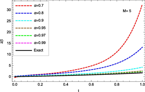
Consider the following PV-FIDE $\begin{matrix} ^{ABC} D_{t}^{α} z (t) = & z (\frac{t}{2}) - 1 + \frac{t^{2}}{4} - \frac{t^{4}}{64} + \frac{t^{5}}{80} - \frac{t^{6}}{384} + t (3 - \frac{1}{2} e^{(- 1 + t) t} - \frac{\sqrt{π} Erfi [\frac{1}{2}]}{4 e^{\frac{1}{4}}}) + \frac{\sqrt{π} tErfi [\frac{1}{2} - t]}{4 e^{\frac{1}{4}}} \\ + \int_{0}^{t} t τ e^{z (τ)} d τ + \int_{0}^{\frac{t}{2}} τ z^{2} (τ) d τ, t \in [0, 1], \end{matrix}$ under the initial condition $z (0) = 0,$ where $Erfi (\cdot)$ is the imaginary error function. The exact solution is given by $z (t) = t^{2} - t$ when $α = 1$ . For different values of $α$ , in Fig. 2, by setting $M = 5, 7$ and $T = 1, 2$ , we have reported the obtained numerical results by the proposed scheme at some selected points. Also, by considering $T = 1$ , comparison of the absolute error at those selected points with different values M and $α$ is shown in Tables 2 and 3.

Example 3

Consider the following PT-FIDE $\begin{matrix} ^{ABC} D_{t}^{α} z (t) = & \frac{1}{2} z (t) + z (\frac{t}{4}) + \frac{1}{2} - \frac{t}{4} e^{\frac{t}{4}} + \frac{t^{2}}{32} - \frac{1}{2} e^{3 t} + e^{2 t} \\ + \int_{0}^{t} e^{t + τ} z (τ) d τ + \int_{0}^{\frac{t}{4}} τ z (τ) d τ, t \in [0, 1], \end{matrix}$ under the initial condition $z (0) = 0 .$ Zhao et al. (2017) have considered this example and solved it by the SCM to achieve its approximate solution. Hence, in Table 4, the MAE of $z (t)$ obtained by the proposed scheme with those obtained in Zhao et al. (2017) at various values of M is compared. Also, by taking $M = 5$ , the approximate solution together with the exact solution ( $z (t) = e^{t} - 1$ when $α = 1$ ) with different choices of $α$ are shown in Fig. 3.

Example 4

Consider the fractional pantograph differential equation $^{ABC} D_{t}^{α} z (t) = - z (t) + 0.1 z (0.2 t) - 0.1 e^{- 0.2 t}, t \in [0, 1],$ under the initial condition $z (0) = 1 .$

By employing the proposed scheme, we have achieve the approximate solution by setting $M = 5$ and plotted the approximate solution along with the exact solution ( $z (t) = e^{- t}$ when $α = 1$ ) at various values of $α$ . This problem is solved with different methods given in Muroya et al. (2003), Rahimkhani et al. (2017), Nemati et al. (2018) which include collocation method, operational matrix based on Bernoulli wavelets and hat functions, respectively. By setting $M = 10, α = 1$ and $T = 1$ , the results obtained are compared with methods given in Muroya et al. (2003), Rahimkhani et al. (2017), Nemati et al. (2018) at some selected points in Table 5. Table 5 shows the proposed scheme gives more favorable results than the method given by Muroya et al. (2003), Rahimkhani et al. (2017), Nemati et al. (2018). Also, comparison of the absolute error at some selected points with different values $α$ is shown in Table 6.

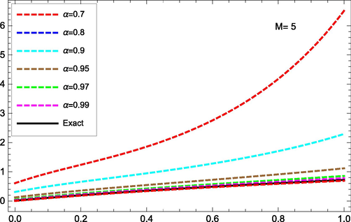
(Example 1) Approximate solutions for different values of α .

Table 1 (Example 1) Comparison of the absolute error at some selected points for

α = 1

	Method of Zhao et al. (2017)		Present method
M	MAE	M	MAE	CPU time
5	1.70e−3	3	9.96e−4	0.016
10	1.11e−4	5	3.62e−5	0.063
20	1.96e−6	7	1.57e−6	0.156
30	8.70e−8	10	5.17e−8	0.516
40	6.26e−9	12	2.50e−9	1.047

(Example 2) The exact and approximate solutions given by different values of α (a) M = 5 and t ∈ [ 0 , 1 ] (b) M = 7 and t ∈ [ 0 , 2 ] .

Table 2 (Example 2) Comparison of the absolute error at some selected points with different values M.

		$α = 1$	$T = 1$
t	$M = 3$	$M = 5$	$M = 7$	$M = 9$	$M = 11$
0.1	1.94e−5	1.20e−6	1.13e−8	2.83e−11	1.62e−12
0.3	2.68e−5	2.73e−7	1.73e−8	1.54e−10	1.44e−12
0.5	8.38e−5	2.25e−6	4.61e−9	2.82e−10	1.19e−12
0.7	1.33e−4	1.41e−6	2.20e−8	6.32e−11	2.57e−12
0.9	5.66e−5	2.06e−6	1.91e−8	3.43e−10	5.13e−13

Table 3 (Example 2) Comparison of the absolute error at some selected points with different values

α

		$M = 7$	$T = 1$
t	$α = 0.7$	$α = 0.8$	$α = 0.9$	$α = 0.99$	$α = 1$
0.1	7.20e−1	3.53e−1	1.37e−2	1.13e−3	1.13e−8
0.3	7.28e−1	3.34e−1	1.22e−2	9.58e−3	1.73e−8
0.5	6.53e−1	2.71e−1	8.78e−2	6.14e−3	4.61e−9
0.7	5.51e−1	1.91e−1	4.54e−2	1.90e−3	2.20e−8
0.9	4.51e−1	1.08e−1	8.75e−5	2.66e−3	1.91e−8

Table 4 (Example 3) Comparison of the absolute error at some selected points for

α = 1

	Method of Zhao et al. (2017)		Present method
M	MAE	M	MAE	CPU time
5	3.60e−3	3	2.30e−3	0.031
10	2.23e−4	5	2.83e−5	0.078
20	5.72e−6	7	1.20e−7	0.406
30	2.89e−7	10	4.50e−10	1.016
40	2.21e−8	12	1.42e−10	2.203

(Example 3) The exact and approximate solutions given by different values of α .

Table 5 (Example 4) Comparison of the absolute errors for

α = 1

	Muroya et al. (2003)	Rahimkhani et al. (2017)	Nemati et al. (2018)	Presented method
t		$M = 32$	$k = 2, M = 6$	$M = 10$
$2^{- 2}$	$1.08 e - 5$	$8.79 e - 9$	$1.05 e - 8$	$2.22 e - 15$
$2^{- 3}$	$3.81 e - 5$	$1.89 e - 8$	$5.79 e - 9$	$2.66 e - 15$
$2^{- 4}$	$1.26 e - 5$	$8.92 e - 9$	$2.00 e - 8$	$3.11 e - 15$
$2^{- 5}$	$4.09 e - 5$	$3.55 e - 8$	$3.70 e - 9$	$7.77 e - 15$
$2^{- 6}$	$1.20 e - 5$	$1.83 e - 6$	$2.03 e - 8$	$4.33 e - 15$

Table 6 (Example 4) Comparison of the absolute error at some selected points with different values

α

		$M = 7$	$T = 1$
t	$α = 0.7$	$α = 0.8$	$α = 0.9$	$α = 0.99$	$α = 1$
0.1	2.68e−1	1.88e−1	9.85e−2	1.02e−3	3.50e−7
0.3	1.95e−1	1.39e−1	7.38e−2	7.75e−3	2.61e−7
0.5	1.20e−1	8.51e−2	4.48e−2	4.67e−3	2.91e−7
0.7	5.70e−2	3.89e−2	1.94e−2	1.90e−3	2.70e−7
0.9	2.22e−3	1.31e−3	2.80e−3	5.38e−4	3.73e−7

7 Conclusion

In this article, an efficient method has been proposed to obtain numerical solution of pantograph Volterra nonlinear fractional integro-differential equations which is described in the Atangana-Baleanu sense. For solving the considered equations, the properties of the shifted Legendre polynomials together with the collocation points have been used. By this way, the problem under study is reduced to a system of algebraic equations which greatly simplifies the problem. Then, an error estimate is proved for the proposed scheme. Finally, some examples have been presented to show the accuracy and efficiency of the proposed scheme. The numerical results confirm the superiority of this method compared to the other existing state of the art methods. see Fig. 4.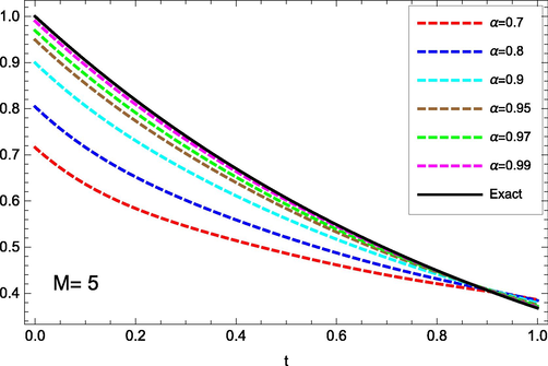

(Example 4) Approximate solutions given by different values of α .

Declaration of Competing Interest

The authors declare that they have no known competing financial interests or personal relationships that could have appeared to influence the work reported in this paper.

References

Ait Touchent K., Hammouch Z., Mekkaoui T., Belgacem F.B.M., . Implementation and convergence analysis of homotopy perturbation coupled with sumudu transform to construct solutions of local-fractional PDEs. Fract. Fraction.. 2018;2(3):22.
[CrossRef] [Google Scholar]
Algahtani O.J.J., . Comparing the Atangana-Baleanu and Caputo-Fabrizio derivative with fractional order: Allen Cahn model. Chaos Solitons Fract.. 2016;89:552-559.
[Google Scholar]
Atangana A., Baleanu D., . New fractional derivatives with nonlocal and non-singular kernel: theory and application to heat transfer model. Therm. Sci.. 2016;20(2):763-769.
[Google Scholar]
Atangana A., Hammouch Z., . Fractional calculus with power law: the cradle of our ancestors. Eur. Phys. J. Plus. 2019;134:429.
[Google Scholar]
Atangana A., Kocab I., . Chaos in a simple nonlinear system with Atangana-Baleanu derivatives with fractional order. Chaos Solitons Fract.. 2016;89:447-454.
[Google Scholar]
Baleanu D., Diethelm K., Scalas E., Trujillo J.J., . Fractional Calculus: Models and Numerical Methods. World Scientific Publishing Company; 2012.
Canuto C., Hussaini M.Y., Quarteroni A., Zang T.A., . Spectral Methods, Scientific Computation. Berlin: Springer-Verlag; 2006.
Caputo M., Fabrizio M., . A new definition of fractional derivative without singular kernel. Prog. Fraction. Different. Appl.. 2015;1(2):73-85.
[Google Scholar]
Djida J.D., Atangana A., Area I., . Numerical computation of a fractional derivative with non-local and non-singular kernel. Math. Model. Nat. Phenom.. 2017;12(3):4-13.
[Google Scholar]
Djordjevic V.D., Jaric J., Fabry B., Fredberg J.J., Stamenovic D., . Fractional derivatives embody essential features of cell rheological behavior. Ann. Biomed. Eng.. 2003;31:692-699.
[Google Scholar]
Deiveegan A., Nieto J.J., Prakash P., . The revised generalized Tikhonov method for the backward time-fractional diffusion equation. J. Appl. Anal. Comput.. 2019;9:45-56.
[Google Scholar]
Ganji R.M., Jafari H., . A new approach for solving nonlinear Volterra integro-differential equations with Mittag-Leffler kernel. Proc. Inst. Math. Mech.. 2020;46(1):144-158.
[Google Scholar]
Ganji R.M., Jafari H., Adem A.R., . A numerical scheme to solve variable order diffusion–wave equations. Therm. Sci.. 2019;23(Suppl. 6):2063-2071.
[CrossRef] [Google Scholar]
Ganji R.M., Jafari H., . Numerical solution of variable order integro-differential equations. Adv. Math. Models Appl.. 2019;4(1):64-69.
[Google Scholar]
Ganji R.M., Jafari H., Baleanu D., . A new approach for solving multi variable orders differential equations with Mittag-Leffler kernel. Chaos Solitons Fract.. 2020;130:109405
[Google Scholar]
Ganji R.M., Jafari H., Nemati S., . A new approach for solving integro-differential equations of variable order. J. Comput. Appl. Math.. 2020;379:112946
[Google Scholar]
Jafari H., Das S., Tajadodi H., . Solving a multi-order fractional differential equation usinghomotopy analysis method. J. King Saud Univ. Sci.. 2011;23(2):151-155.
[Google Scholar]
Jothimani K., Kaliraj K., Hammouch Z., Ravichandran C., . New results on controllability in the framework of fractional integro-differential equations with nondense domain. Eur. Phys. J. Plus. 2019;134:144.
[Google Scholar]
Khan M.A., Atangana A., . Modeling the dynamics of novel coronavirus (2019-nCov) with fractional derivative. Alexand. Eng. J. 2020
[CrossRef] [Google Scholar]
Losada J., Nieto J.J., . Properties of a new fractional derivative without singular kernel. Prog. Fraction. Differ. Appl.. 2015;1(2):87-92.
[Google Scholar]
Mishra V., Das S., Jafari H., Ong S.H., . Study of fractional order Van der Pol equation. J. King Saud Univ. Sci.. 2016;28(1):55-60.
[Google Scholar]
Muroya Y., Ishiwata E., Brunner H., . On the attainable order of collocation methods for pantograph integro-differential equations. J. Comput. Appl. Math.. 2003;152:347-366.
[Google Scholar]
Nemati S., Lima P., Sedaghat S., . An effective numerical method for solving fractional pantograph differential equations using modification of hat functions. Appl. Numer. Math.. 2018;131:174-189.
[Google Scholar]
Nieto J.J., Samet B., . Solvability of an implicit fractional integral equation via a measure of noncompactness argument. Acta Math. Sci.. 2017;37(1):195-204.
[Google Scholar]
Podlubny I., . Fractional Differential Equations. San Diego: Academic Press; 1999.
Rahimkhani P., Ordokhani Y., Babolian E., . A new operational matrix based on Bernoulli wavelets for solving fractional delay differential equations. Numer. Algor.. 2017;74(1):223-245.
[Google Scholar]
Sabermahani S., Ordokhani Y., Yousefi S.A., . Numerical approach based on fractional-order Lagrange polynomials for solving a class of fractional differential equations. Comput. Appl. Math.. 2018;37:3846-3868.
[Google Scholar]
Sabermahani S., Ordokhani Y., Yousefi S.A., . Fractional-order Fibonacci-hybrid functions approach for solving fractional delay differential equations. Eng. Comput.. 2020;36:795-806.
[Google Scholar]
Sedaghat S., Ordokhani Y., Dehghan M., . On spectral method for Volterra functional integro-differential equations of neutral type. Numer. Function. Anal. Optim.. 2014;35(2):223-239.
[CrossRef] [Google Scholar]
Singh H., Srivastava H.M., . Jacobi collocation method for the approximate solution of some fractional-order Riccati differential equations with variable coefficients. Phys. A Stat. Mech. Appl.. 2019;523:1130-1149.
[Google Scholar]
Srivastava H.M., Raina R.K., Yang X.J., . Special Functions in Fractional Calculus and Related Fractional Differintegral Equations. World Scientific; 2021.
Srivastava H.M., Shah F.A., Abass R., . An application of the Gegenbauer wavelet method for the numerical solution of the fractional Bagley-Torvik Equation. Russ. J. Math. Phys.. 2019;26:77-93.
[Google Scholar]
Tajadodi H., . A Numerical approach of fractional advection-diffusion equation with Atangana-Baleanu derivative. Chaos Solitons Fract.. 2020;130:109527
[Google Scholar]
Yang X.J., . General Fractional Derivatives: Theory, Methods and Applications. New York: CRC Press; 2019.
Yang X.J., Gao F., Yang J., . General Fractional Derivatives with Applications in Viscoelasticity. Academic Press; 2020.
Yang X.J., Abdel-Atya M., Cattani C., . A new general fractional-order derivative with Rabotnov fractional exponential kernel applied to model the anomalous heat transfer. Therm. Sci.. 2019;23(3A):1677-1681.
[Google Scholar]
Yang X.J., Gao F., Yang J., Zhou H.W., . Fundamental solutions of the general fractional-order diffusion equations. Math. Methods Appl. Sci.. 2018;41(18):9312-9320.
[Google Scholar]
Yang X.J., Tenreiro Machado J.A., . A new fractional operator of variable order: application in the description of anomalous diffusion. Phys. A Stat. Mech. Appl.. 2017;481:276-283.
[Google Scholar]
Zhao J., Cao Y., Xu Y., . Sinc numerical solution for pantograph Volterra delay-integro-differential equation. Int. J. Comput. Math.. 2017;94(5):853-865.
[Google Scholar]
Ziane D., Baleanu D., Belghaba K., Cherif M.H., . Local fractional Sumudu decomposition method for linear partial differential equations with local fractional derivative. J. King Saud Univ. Sci.. 2019;31(1):83-88.
[Google Scholar]

Introduction

RL and AB operators and their properties

The SLPs and their properties

The SLPs
Approximation of a function

Numerical scheme

Error estimation

Numerical results

Conclusion

Declaration of Competing Interest

Fulltext Views
4

PDF downloads
0

View/Download PDF
Download Citations

BibTeX
RIS

Show Sections

[1] Ait Touchent K., Hammouch Z., Mekkaoui T., Belgacem F.B.M., . Implementation and convergence analysis of homotopy perturbation coupled with sumudu transform to construct solutions of local-fractional PDEs. Fract. Fraction.. 2018;2(3):22.
[CrossRef] [Google Scholar]

[2] Algahtani O.J.J., . Comparing the Atangana-Baleanu and Caputo-Fabrizio derivative with fractional order: Allen Cahn model. Chaos Solitons Fract.. 2016;89:552-559.
[Google Scholar]

[3] Atangana A., Baleanu D., . New fractional derivatives with nonlocal and non-singular kernel: theory and application to heat transfer model. Therm. Sci.. 2016;20(2):763-769.
[Google Scholar]

[4] Atangana A., Hammouch Z., . Fractional calculus with power law: the cradle of our ancestors. Eur. Phys. J. Plus. 2019;134:429.
[Google Scholar]

[5] Atangana A., Kocab I., . Chaos in a simple nonlinear system with Atangana-Baleanu derivatives with fractional order. Chaos Solitons Fract.. 2016;89:447-454.
[Google Scholar]

[6] Baleanu D., Diethelm K., Scalas E., Trujillo J.J., . Fractional Calculus: Models and Numerical Methods. World Scientific Publishing Company; 2012.

[7] Canuto C., Hussaini M.Y., Quarteroni A., Zang T.A., . Spectral Methods, Scientific Computation. Berlin: Springer-Verlag; 2006.

[8] Caputo M., Fabrizio M., . A new definition of fractional derivative without singular kernel. Prog. Fraction. Different. Appl.. 2015;1(2):73-85.
[Google Scholar]

[9] Djida J.D., Atangana A., Area I., . Numerical computation of a fractional derivative with non-local and non-singular kernel. Math. Model. Nat. Phenom.. 2017;12(3):4-13.
[Google Scholar]

[10] Djordjevic V.D., Jaric J., Fabry B., Fredberg J.J., Stamenovic D., . Fractional derivatives embody essential features of cell rheological behavior. Ann. Biomed. Eng.. 2003;31:692-699.
[Google Scholar]

[11] Deiveegan A., Nieto J.J., Prakash P., . The revised generalized Tikhonov method for the backward time-fractional diffusion equation. J. Appl. Anal. Comput.. 2019;9:45-56.
[Google Scholar]

[12] Ganji R.M., Jafari H., . A new approach for solving nonlinear Volterra integro-differential equations with Mittag-Leffler kernel. Proc. Inst. Math. Mech.. 2020;46(1):144-158.
[Google Scholar]

[13] Ganji R.M., Jafari H., Adem A.R., . A numerical scheme to solve variable order diffusion–wave equations. Therm. Sci.. 2019;23(Suppl. 6):2063-2071.
[CrossRef] [Google Scholar]

[14] Ganji R.M., Jafari H., . Numerical solution of variable order integro-differential equations. Adv. Math. Models Appl.. 2019;4(1):64-69.
[Google Scholar]

[15] Ganji R.M., Jafari H., Baleanu D., . A new approach for solving multi variable orders differential equations with Mittag-Leffler kernel. Chaos Solitons Fract.. 2020;130:109405
[Google Scholar]

[16] Ganji R.M., Jafari H., Nemati S., . A new approach for solving integro-differential equations of variable order. J. Comput. Appl. Math.. 2020;379:112946
[Google Scholar]

[17] Jafari H., Das S., Tajadodi H., . Solving a multi-order fractional differential equation usinghomotopy analysis method. J. King Saud Univ. Sci.. 2011;23(2):151-155.
[Google Scholar]

[18] Jothimani K., Kaliraj K., Hammouch Z., Ravichandran C., . New results on controllability in the framework of fractional integro-differential equations with nondense domain. Eur. Phys. J. Plus. 2019;134:144.
[Google Scholar]

[19] Khan M.A., Atangana A., . Modeling the dynamics of novel coronavirus (2019-nCov) with fractional derivative. Alexand. Eng. J. 2020
[CrossRef] [Google Scholar]

[20] Losada J., Nieto J.J., . Properties of a new fractional derivative without singular kernel. Prog. Fraction. Differ. Appl.. 2015;1(2):87-92.
[Google Scholar]

[21] Mishra V., Das S., Jafari H., Ong S.H., . Study of fractional order Van der Pol equation. J. King Saud Univ. Sci.. 2016;28(1):55-60.
[Google Scholar]

[22] Muroya Y., Ishiwata E., Brunner H., . On the attainable order of collocation methods for pantograph integro-differential equations. J. Comput. Appl. Math.. 2003;152:347-366.
[Google Scholar]

[23] Nemati S., Lima P., Sedaghat S., . An effective numerical method for solving fractional pantograph differential equations using modification of hat functions. Appl. Numer. Math.. 2018;131:174-189.
[Google Scholar]

[24] Nieto J.J., Samet B., . Solvability of an implicit fractional integral equation via a measure of noncompactness argument. Acta Math. Sci.. 2017;37(1):195-204.
[Google Scholar]

[25] Podlubny I., . Fractional Differential Equations. San Diego: Academic Press; 1999.

[26] Rahimkhani P., Ordokhani Y., Babolian E., . A new operational matrix based on Bernoulli wavelets for solving fractional delay differential equations. Numer. Algor.. 2017;74(1):223-245.
[Google Scholar]

[27] Sabermahani S., Ordokhani Y., Yousefi S.A., . Numerical approach based on fractional-order Lagrange polynomials for solving a class of fractional differential equations. Comput. Appl. Math.. 2018;37:3846-3868.
[Google Scholar]

[28] Sabermahani S., Ordokhani Y., Yousefi S.A., . Fractional-order Fibonacci-hybrid functions approach for solving fractional delay differential equations. Eng. Comput.. 2020;36:795-806.
[Google Scholar]

[29] Sedaghat S., Ordokhani Y., Dehghan M., . On spectral method for Volterra functional integro-differential equations of neutral type. Numer. Function. Anal. Optim.. 2014;35(2):223-239.
[CrossRef] [Google Scholar]

[30] Singh H., Srivastava H.M., . Jacobi collocation method for the approximate solution of some fractional-order Riccati differential equations with variable coefficients. Phys. A Stat. Mech. Appl.. 2019;523:1130-1149.
[Google Scholar]

[31] Srivastava H.M., Raina R.K., Yang X.J., . Special Functions in Fractional Calculus and Related Fractional Differintegral Equations. World Scientific; 2021.

[32] Srivastava H.M., Shah F.A., Abass R., . An application of the Gegenbauer wavelet method for the numerical solution of the fractional Bagley-Torvik Equation. Russ. J. Math. Phys.. 2019;26:77-93.
[Google Scholar]

[33] Tajadodi H., . A Numerical approach of fractional advection-diffusion equation with Atangana-Baleanu derivative. Chaos Solitons Fract.. 2020;130:109527
[Google Scholar]

[34] Yang X.J., . General Fractional Derivatives: Theory, Methods and Applications. New York: CRC Press; 2019.

[35] Yang X.J., Gao F., Yang J., . General Fractional Derivatives with Applications in Viscoelasticity. Academic Press; 2020.

[36] Yang X.J., Abdel-Atya M., Cattani C., . A new general fractional-order derivative with Rabotnov fractional exponential kernel applied to model the anomalous heat transfer. Therm. Sci.. 2019;23(3A):1677-1681.
[Google Scholar]

[37] Yang X.J., Gao F., Yang J., Zhou H.W., . Fundamental solutions of the general fractional-order diffusion equations. Math. Methods Appl. Sci.. 2018;41(18):9312-9320.
[Google Scholar]

[38] Yang X.J., Tenreiro Machado J.A., . A new fractional operator of variable order: application in the description of anomalous diffusion. Phys. A Stat. Mech. Appl.. 2017;481:276-283.
[Google Scholar]

[39] Zhao J., Cao Y., Xu Y., . Sinc numerical solution for pantograph Volterra delay-integro-differential equation. Int. J. Comput. Math.. 2017;94(5):853-865.
[Google Scholar]

[40] Ziane D., Baleanu D., Belghaba K., Cherif M.H., . Local fractional Sumudu decomposition method for linear partial differential equations with local fractional derivative. J. King Saud Univ. Sci.. 2019;31(1):83-88.
[Google Scholar]

A new numerical scheme for solving pantograph type nonlinear fractional integro-differential equations

Abstract

Keywords

Non-local and non-singular kernel

Volterra nonlinear fractional integro-differential equations

Atangana–Baleanu operator

The shifted Legendre polynomials

Approximation solution

34A08

65M70

11B68

1 Introduction

2 RL and AB operators and their properties

Definition 1 See Podlubny (1999)

Definition 2 See Podlubny (1999)

Definition 3 See Atangana and Baleanu (2016), Yang (2019)

Theorem 1 See Tajadodi (2020)

3 The SLPs and their properties

3.1 The SLPs

3.2 Approximation of a function

Lemma 2 See Ganji et al. (2020)

4 Numerical scheme

5 Error estimation

Lemma 3 See Canuto et al. (2006)

Lemma 4 See Ganji et al. (2020)

6 Numerical results

7 Conclusion

Declaration of Competing Interest

References

Suggested read for related articles: