

Translate this page into:
Exponentiated odd Lindley-X family with fitting to reliability and medical data sets
⁎Corresponding author. ahmed.abdelbar@science.tanta.edu.eg (Ahmed M. T. Abd El-Bar)
-
Received: ,
Accepted: ,
This article was originally published by Elsevier and was migrated to Scientific Scholar after the change of Publisher.
Peer review under responsibility of King Saud University.
Abstract
This paper concerns constructing a general family of distributions called exponentiated odd Lindley-X (EOL-X) family. We demonstrate that the EOL-X density can be represented as an infinite linear combination of the exponentiated-F densities and, as a result, that many of its mathematical features are derived directly. The fundamental statistical properties, including moments, mean deviations, generating function, order statistics, stochastic ordering, and entropies were investigated. EOL-X special models are introduced. The suggested model presents superior performance when compared to the other models studied, in the reliability and “medical” data. In addition, its bimodal density shape enhances the possibility of good tuning in applications in several other areas, such as survival. Thus, it is expected that this proposal will be of great help to the community studying new families and their adjustments to real data sets.
Keywords
Exponentiated odd Lindley
Moments
Medical data set
Reliability data set
Survival data set

1 Introduction
The most diverse distributions proposed in the literature are extremely important for understanding and modeling real data. Unfortunately, it has not yet been proposed a family of distributions that satisfactorily fits the phenomena studied in all areas of knowledge. For this reason, more and more researchers are dedicated to proposing new models that have a better fit in certain cases when compared to other models previously established in the literature. Over the decades, many families have been proposed. Below, we cite a few: Gleaton and Lynch (Gleaton and Lynch, 2006) proposed the generator odd-log-logistic-G; Alexander et al. (Alexander et al., 2012) developed the class Generalized Beta-Generated, among others.
More recently, some new families are proposed using the generator of families proposed by Alzaatreh et al. (Alzaatreh et al., 2013). For example, Ferreira (Ferreira, 2021), using this generator, proposed and studied the Quasi-Lindley-X family of distributions.
In addition, studies with combinations between transformations and this generator have also been carried out, such as the work done by Klakattawi et al. (Klakattawi et al., 2022), where the authors combine the Marshall-Olkin transformation with the T-X family of distributions.
Therefore, based on the knowledge that the Lindley distribution and its extensions have been shown to be quite adequate in modeling “medical” data sets, we seek to motivate the choice of the generator of families of T-X distributions, using the exponentiated odd Lindley, and we will see that this family can, depending on the baseline, embody at least three of the four important forms for the risk function, namely: increasing, decreasing and bathtub. This constitutes an important point of the family, since it allows a better suitability for different types of data set.
Recently, Alzaatreh et al. (Alzaatreh et al., 2013) have introduced the T-X family as
Moreover, the exponentiated T-X family proposed by Alzaghal et al. (Alzghal et al., 2013). In addition, Gomes-Silva et al. (Gomes-Silva et al., 2017) described the odd Lindley-G family. In this work, we will develop some mathematical properties of one member of the exponentiated odd S-X family which is also a general family of distributions, namely the exponentiated odd Lindley-X (EOL-X) family and illustrate the versatility of the EOL-X family to fit and model real data. Various shapes of the hazard rate function (hrf) and density of sub-models for EOL-X family support the family to fit several real lifetime data which represent one of the motivations to the family beside others that will be mention through the paper, such as mixture representation of the density and cdf of the family in terms of exp-F distributions.
Next, we give some remarks and properties on the EOS-X family.
Replacing by in (1), we have the cdf of the EOS-X.
The hrf of the EOS-X is
Let follows the EOS-X family (3), the associated quantile function is.
Let follows the EOS-X family with the pdf (3), then the Shannon entropy (SE) of is.
Note that, (2) and (3) do not involve any complicated functions. Thus, if we choose distributions with simple density for S, we will have a family of distributions with density and cumulative functions of easy mathematical and computational treatment, when compared with families such as gamma-G and beta-G, for example. Besides that, we can note that (3) provide distribution families generators, depend on the choice of S. In this way, this work ‘opens the doors’ to proposals of new distributions with density in the form (3). Here, we choose by the simplicity of its pdf.
To demonstrate the effectiveness of the proposed model, we study its fit to three real data sets. The first one address the failure time of turbochargers, components play an important role in the safe operation of merchant vessels, since they play a key role in the proper functioning of the main engine. This data is presented in application section. Some papers have been studied the use of some distributions through the adjustment of this data: Singla et. al. (Singla et al., 2012) show that the beta generalized Weibull model is preferable over its sub models using this data set and Benkhelifa (Benkhelifa, 2020) demonstrate the flexibility to the Weibull Birnbaum-Saunders distribution by means this data.
In order to show the flexibility of the proposal to different situations, we also include applications to survival data. In addition, we know that many of the families that are part of the S-X family are well suited to these types of sets. In this sense, the second data constitutes a survival data set, since each observation is the time to death (in months) of patients with breast cancer with different immuno-biochemical responses (for more details, see Klein and Moeschberger (Klein and Moeschberger, 2005).
It is important to study breast cancer data since this type of cancer is one of the most frequent in women around the world. It is the most common in women in the United States. In Brazil, it only loses to non-melanoma skin and accounts for 29 % of new cases each year, according to the National Cancer Institute.
The third data is a study about Aids clinical trial nested and can be found in https://www.umass.edu/statdata/statdata/stat-survival.html. Clinical studies with Aids data are of great relevance in the scientific and social aspects. Despite being a disease already known worldwide since the early 1980 s, there is still a lot of prejudice and, in some countries, lack of access to information and medicines.
Brazil has stood out, among other aspects, with programs for the distribution of condoms and antiretroviral drugs at no additional cost. Although programs like these have not eradicated such an epidemic, they help increase patient survival and quality of life. Much still needs to be done to heal healing, and statistical study is an important tool in this process.
The following is a list of the paper's supplements. We propose the exponentiated odd Lindley-X family and some of its sub-models, in Section 2. In Section 3, we show the mixture representation of the density and cdfs of the family. We provide various of the new family’s mathematical features in Section 4. Stochastic ordering and the two popular entropies are investigated in Sections 5 and 6, respectively. An estimation procedure for EOL-X parameters is obtained in Section 7. Simulation studies are provided in Section 8. We chose some data sets to evaluate the performance of sub-model of the family using a set of goodness-of-fit statistics in Section 9. Finally, some conclusions about the obtained results are reported in Section 10.
2 EOL-X family with sub-models
The EOL-X family is proposed in this section. Some sub-models of the family are given and it is observed that their pdfs could be unimodal, left-skewed, right-skewed, bimodal and their hrfs could be bathtub, decreasing, constant, increasing, J and reversed-J shaped. All this gains the family much flexibility for fitting and modeling real life data.
2.1 The EOL-X family
Let S follows the Lindley distribution with pdf
, then the pdf of the EOL-X family using (3) is
where
is a baseline cdf depending on a parameter vector
By using (2) and the cdf of the Lindley distribution,
The EOL-X family's cdf can be found here
Hence, the hrf of
is
2.2 Sub-models
Some sub-models in the EOL-X family (7) are given in function of three well-known distributions; exponential (E) with cdf Lomax (Lo) with cdf defined as and Dagum (Da) with cdf .
2.2.1 The EOL-E distribution
Using the exponential pdf and cdf as input for (7) and (9), we get the EOL-E pdf and hrf.
and
respectively. The pdf and hrf of EOL-E are plotted in Fig. 1 for distinct parameters values.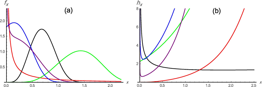
Plots of the EOL-E pdf and hrf. (a)
(black),
(red),
(green),
(blue),
(purple).(b)
(green),
(black),
(blue),
(red),
(Purple).
2.2.2 The EOL-Lo distribution
Inserting the Lomax pdf and cdf as input for (7) and (9), implies the EOL-Lo pdf and hrf as
respectively. Fig. 2 shows plots of the pdf and hrf of the EOL-Lo for the specified parameter values.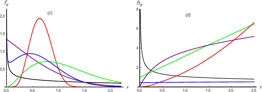
Plots of the EOL-Lo pdf and hrf. (c)
(black),
(red),
(green),
(purple),
(blue)(d)
(green),
(black),
(purple),
(blue),
(red),
2.2.3 The EOL-Da distribution
Taking the Dagum pdf and cdf as input for (7) and (9), the following functions hold
and
The pdf and hrf curves of the EOL-Da model are displayed in Fig. 3.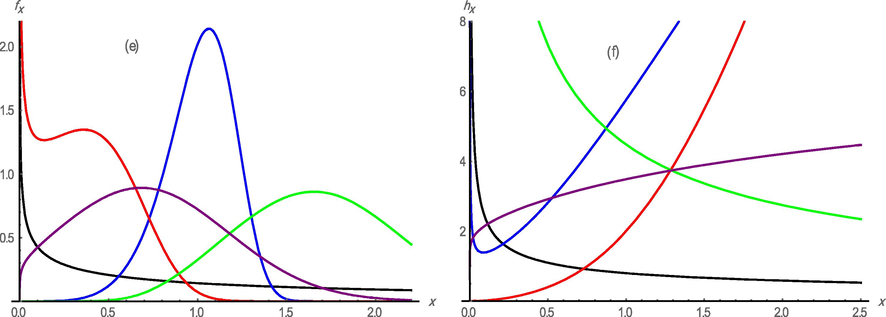
Plots of the EOL-D pdf and hrf. (e)
(black),
(blue),
(red),
(green),
(pruple). (f)
(black),
(blue),
(green),
(red),
(purple).
3 Expansions for the EOL-X family
This section displays a mixture representation of the EOL-X family's pdf and cdf. This family's quantile function is also provided.
3.1 Expansion for the dansity function
By making of the power series for the following term, we get
Applying (16) in (7), we have
We should use the generalized binomial theorem to find
Inserting (18) in (17), the pdf (7) can be stated as
and .
Hence, the pdf of the EOL-X family can be expressed as an infinite linear combination of the exponentiated-F (exp-F) density. As a result, the exp-F distribution may be used to derive several mathematical features of EOL-X. Nadarajah and Kotz (Nadarajah and Kotz, 2006) investigate several mathematical features of exp-F distributions.
Then, the mixture representations of the cdf and hrf of EOL-X family are presented, respectively, as
and
3.2 Quantile function
The quantile function,
for the EOL-X family is obtained by using (6) and (8) as
4 Mathematical properties
The mathematical properties of the distributions are important characteristics and must be obtained, whenever possible, in a closed form, that is, in function of known mathematical functions. However, we know that often proposing new distributions brings with it the problem of obtaining such properties in this format. Therefore, when we can express the density and distribution functions as a linear mixture of accumulated densities, respectively, of the exponential distributions-G, we use power series properties to obtain these results.
In this sence, we intrduced various mathematical features of the EOL-X family in this section, including moments, mean deviations, generating function, (reversed) residual lifetime moments and order statistics.
4.1 Moments
Using (19) and the definition of the nth moment about the origin of
we have
The baseline quantile function can be used as another formulation for as follows:
Using (19), we can write
as
Cordeiro and Nadarajah (Cordeiro and Nadarajah, 2011) obtained for some well-known distributions which can be used to determine the EOL-X moments.
4.2 Incomplete moments
The nth incomplete moment of
is given by
4.3 Moment generating function
The moment generating function (mgf) of the EOL-X family is presented two expressions here. The first one can be obtained from the Exp-F mgf as
4.4 Mean deviations
The mean deviations about the mean (
) and about the median (
) of the EOL-X family can be obtained as.
respectively, where
is obtained from (23),
is the median of
and
is obtained from (21) and (22),
is evaluated by the cdf of the EOL-X family and
is the first incomplete moment can be obtained from (19) as
4.5 Moments of residual and reversed residual lifetime
The moments of residual and reversed residual lifetime of the EOL-X family are given by
and
respectively, where and are the cdf and survival function of the EOL-X family, given by (23), and is the nth incomplete moment given by (25).
4.6 Order statistics
The pdf of the ith order statistic, say
for a random sample
from the EOL-X family is given by
Inserting (7) and (8) into (32), the
becomes
and denotes the EOL-X pdf with parameters and
5 Stochastic ordering
The EOL-X family is ordered in terms of likelihood ratio ordering, as shown by the next theorem.
Let EOL-X and EOL-X If then is stated to be smaller than in the likelihood ratio order (denoted by ).
Proof. The likelihood ratio is given by
Since
Hence is decreasing in That is which completes the proof.
6 Entropies
Here, we discuss two common entropy measures that are the Shannon entropy and Rényi entropy. In what follows, we derive two entropies of the EOL-X family.
The EOL- family's Shannon entropy (SE) is given by.
Proof. The proof follows from Remark 4 and the SE for the Lindley distribution:
which is given by Ghitany et al. (Ghitany et al., 2008).
The EOL- family's Rényi entropy is described by
where the coefficients .
Proof. Using the definition of Rényi entropy and the pdf (7), hence
Applying (16) in the expression above, we have
Therefore, desired proof is obtained by expanding the binomial term in the integral above.
7 Inference on the EOL-X family parameters
An estimation procedure for EOL-X parameters are discussed here.
Let be observed values from the EOL-X defined by (7) with parameter vector Then, the log-likelihood function for is
The elements of the score vector are
and where Equating and with zero, as well as numerically solving these equations, then the MLEs of are obtained.
8 Simulation study
Here, we present a simulation analysis to demonstrate the MLEs parameters vector's asymptotic behavior. To do this, we choose the sub-model EOLE, defined in (10). Using the R software, we execute a Monte Carlo simulation study, with 1000 replications. Setting
and
, The MLEs' accuracy is measured. Aside from that, we use the random censoring system on the right to censor percentages (
and
) and
, and
. As a result, we present the MLEs' average estimates (AEs) as well as the mean squared errors (MSEs), for each parameter point. The results in Table 1 show that the sufficiency condition is valid and that the estimators are consistent.
Parameter
AE
MSE
AE
MSE
AE
MSE
1.002
0.007
1.091
0.017
1.078
0.014
2.030
0.054
1.828
0.074
1.850
0.066
3.048
0.007
2.764
0.122
2.798
0.105
1.002
0.003
1.097
0.014
1.079
0.010
2.008
0.027
1.800
0.059
1.842
0.046
3.016
0.039
2.724
0.105
2.789
0.075
1.007
0.002
1.086
0.010
1.073
0.007
2.009
0.017
1.815
0.048
1.848
0.036
3.016
0.025
2.746
0.084
2.793
0.062
9 Applications to modeling reliability and medical data
Here, we compare the performance of the EOLE model at Subsection 2.2 to a set of classical and recent lifetime distributions.
The lifetime distributions used in comparison are:
-
Gamma (Ga) distribution;
-
Lindley– exponential (LE) distribution – Bhati et al. (Bhati et al., 2015);
-
Transmuted exponentiated Exponential (TEE) distribution – Merovci (Merovci, 2013);
-
Beta exponential (BE) – Nadarajah and Kotz (Nadarajah and Kotz, 2006);
-
Gamma-exponentiated exponential (GEE) distribution–Ristic' and Balakrishnan (Ristic' and Balakrishnan, 2012);
-
Transmuted exponentiated Lomax (TELo) distribution – Ashour and Eltehiwy (Ashour and Eltehiwy, 2013);
-
Gamma-Dagum (GDa) distribution – Oluyede et al. (Oluyede et al., 2014);
-
Modified Weibull (MW) distribution – Sarhan and Zaindin (Sarhan and Zaindin, 2009);
-
Genralized Beta Generated Lindley (GBGL) distribution – Lima et al. (Lima et al., 2017);
-
Gamma Lindley (GL) distribution –Lima (Lima, 2015).
For comparison purposes, we consider some real data sets in many areas. The main aim here is to show that our proposed model fits well several types of data. The first piece of data reflects the time it takes for a turbocharger to fail (103h), see Xu et al. (Xu et al., 2003). The second one lists the time to death (in months) of patients with breast cancer with different immuno-bistochemical responses (for more details, see Klein and Moeschberger (Klein and Moeschberger, 2005). In this case, we consider all the observations as uncensored observation. The third data is a study about aids clinical trial nested. For each distribution, we get the maximum-likelihood estimate, AIC, BIC, HQIC, W* and A* goodness-of-fit statistics. To do this, we use the function goodness.fit from software R, with the SANN method. Besides that, the initial kicks were obtained through a heuristic method with the GenSA. Table 2 gives some descriptive statistics for all data sets. The first data is left skewed and while the rest of the data sets are right skewed. The obtained results are presented in Tables 3-8. We developed different situations depend on each application. As we can see the EOLE is powerful competitor to the compared distributions. Moreover, the least values for the considered goodness-of-fit statistics are achieved for EOLE model. The EOLE model performed the best, as predicted from the previous findings.
Real data sets
Statistics
Data1
Data 2
Data 3
Mean
6.2525
97.02
234.7
Median
6.5
87.5
265
SD
1.95553
51.679
93.854
MD-Mean
1.58723
45.70
78.282
MD-Median
4.73251
46.613
72.278
Kurtosis
− 0.42501
−1.4923
−0.28969
Skewness
− 0.65422
0.03268
0.898730
Model
Parameter estimates
EOLE
3.2056
0.32662
0.42819
BE
7.87221
6.22419
0.13779
TEE
7.59178
0.31855
0.98999
GEE
10.5505
0.10895
8.11926
Ga
7.72269
0.809627
–
LE
10.3036
0.448709
–
GTLo
2749.69
6107.18
9.52379
0.000025
0.318372
GDa
4.16258
0.50276
10.0245
10.116
1.64758
TELo
10.3998
17.4909
0.0332954
−0.63111
–
Model
W*
A*
AIC
BIC
HQIC
EOLE
0.108498
0.36417
166.663
171.73
168.495
Ga
0.209882
1.3834
178.821
182.198
180.042
LE
0.286773
1.8008
184.47
187.848
185.691
TEE
0.218098
1.43834
182.226
187.292
184.058
BE
0.214219
1.41121
181.387
186.454
183.219
GEE
0.221483
1.4507
181.352
186.752
183.517
TELo
0.232215
1.59486
187.744
194.499
190.186
GTLo
0.28377
1.78423
190.3
198.744
193.353
GD
0.701105
3.71635
207.196
215.64
210.249
Model
Parameter estimates
EOLE
1.76770 (0.43848)
1.26683 (0.196734)
0.01077 (0.00166)
TEE
0.02017 (0.00314)
2.91307 (0.89602)
− 0.28051 (0.1745)
EL
1.51417 (0.26956)
0.027508 (0.01339)
1.06001 (0.19539)
MW
1.979 (8.878 e-04)
1000 (5.606 e-02)
7.90e-02 (1.19e-02)
GL
1.60462 (0.37948)
0.029136 (0.00590)
–
LE
3.80833 (0.84147)
0.018864 (0.00300)
–
Ga
2.92634 (0.58952)
0.030165 (0.006621)
–
GBGL
2.108e-01 (1.22e-04)
3.50 (1.186e-01)
6.81e-02 (1.025e-02)
4.41(3.3e-04)
Model
AIC
BIC
HQIC
EOLE
0.183436
1.022546
470.5342
475.886
472.5192
TEE
0.269836
1.701178
654.1809
659.533
656.1659
EL
0.255858
1.615608
557.669
563.022
559.6546
GL
0.207078
1.250375
473.8735
477.441
475.1968
LE
0.213885
1.310178
475.1699
478.738
476.4932
Ga
0.206380
1.244549
473.7209
477.289
475.0442
GBGL
0.209680
1.270334
478.3606
485.497
481.0073
MW
0.195096
1.126919
473.0868
478.439
475.0717
Model
Parameter estimates
EOLE
2.56233 (0.14177)
5.03795 (0.53734)
0.002812 (0.00011)
TEE
0.00859 (0.00031)
2.43428 (0.17779)
− 0.69730 (0.04102)
EL
1.11825 (0.04300)
0.00956 (0.00064)
0.94001 (0.02197)
GL
1.50407 (0.09379)
0.011478 (0.00061)
–
LE
7.99877 (0.63588)
0.011179 (0.00045)
–
Ga
2.95143 (0.16142)
0.012589 (0.00071)
–
Model
AIC
BIC
HQIC
EOLE
5.99974
33.17757
7022.502
7035.57
7027.598
TEE
12.74718
67.79268
11599.84
11612.8
11604.9
EL
7.534813
41.42356
7200.168
7213.23
7205.264
GL
7.980831
43.6366
7161.384
7170.09
7164.782
LE
9.525479
51.5472
7515.95
7524.662
7519.348
Ga
7.93374
43.34001
7158.165
7166.877
7161.562
Also, Fig. 4 shows the TTT plots for all data sets considered here. These plots indicate an increasing hrf (first, second and third data sets) and then reveal the adequacy of the some sub-models of our family to fit these data.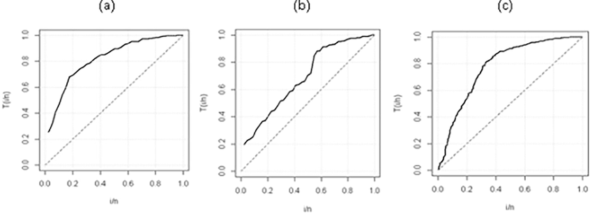
TTT plot for: (a) the first data, (b) second data (c) third data.
Finally, we can conclude that the model studied in this section (using the exponential as a baseline) presents superior performance when compared to the competitive models chosen in the three applications in question. In addition, it is worth mentioning that in the applications studied, the proposed model also presented a better fit when compared to the gamma model.
10 Conclusions
We introduced a new distributions family from the T-X termed exponentiated odd Lindley – X (EOL-X) in this study. A linear representation of the new family's density function makes it simple to determine some of its properties. We developed a mathematical treatment of some sub-models of EOL-X. Besides that, several of their mathematical properties are derived. A simulation study based on the exponentiated odd Lindley exponential was provided. Finally, applications of sub-model of the potential family to three real data evidencing that the EOL-X routinely outperforms other well-known models in the literature. We hope that this research will be useful in a number of areas and that further research will emerge. As future works, the proposed distribution might also be investigated as a bivariate extension, which would likely be a discrete case. Finally, given our suggested model, we may do regression analysis.
Declaration of Competing Interest
The authors declare that they have no known competing financial interests or personal relationships that could have appeared to influence the work reported in this paper.
References
- Generalized beta-generated distributions. Comput. Stat. Data Anal.. 2012;56:1880-1897.
- [Google Scholar]
- A new method for generating families of continuous distributions. Metron. 2013;71:63-79.
- [Google Scholar]
- Exponentiated T-X family of distributions with some applications. Int. J. Statist. Probab.. 2013;2:31-49.
- [Google Scholar]
- Transmuted exponentiated Lomax distribution. Austr. J. Bas. Appl. Sci.. 2013;7:658-667.
- [Google Scholar]
- The Weibull Birnbaum-Saunders Distribution: Properties and Applications. Statistics, Optimization and Information Computing 9; 2020. p. :61-81.
- Lindley-exponential distribution: properties and applications. Metron. 2015;73:335-357.
- [Google Scholar]
- Closed-form expressions for moments of a class of beta generalized distributions. Braz. J. Probab. Statist.. 2011;25:14-33.
- [Google Scholar]
- A proposta de uma família de distribuições aplicada a dados virais brasileiros incluindo o novo Coronavírus. Completion. In: of course work presented to the. Department of Statistics of UFPE; 2021.
- [Google Scholar]
- Properties of generalized log-logistic families of lifetime distributions. J. Probability Statist. Sci.. 2006;4(1):51-64.
- [Google Scholar]
- A new generalized family of distributions based on combining Marshall-Olkin transformation with T-X family. PLoS One. 2022;17(2):e0263673.
- [Google Scholar]
- Survival Analysis: Techniques for Censured and Truncated data. Springer; 2005.
- A new model for describing remission times: the generalized beta-generated Lindley distribution. Ann. Braz. Acad. Sci.. 2017;89:1343-1367.
- [Google Scholar]
- Mathematical properties of some generalized gamma models. Doctoral thesis. Recife: Universidad Federal de Pernambuco; 2015.
- Transmuted exponentiated exponential distribution. Math. Sci. Appl. E-Notes. 2013;1:112-122.
- [Google Scholar]
- A new class of generalized Dagum distribution with applications to income and lifetime data. J. Statist. Econ. Meth.. 2014;3:125-151.
- [Google Scholar]
- The gamma-exponentiated exponential distribution. J. Statist. Comput. and Simul.. 2012;82:1191-1206.
- [Google Scholar]
- The Beta Generalized Weibull distribution: Properties and applications. Reliab. Eng. Syst. Saft.. 2012;102:5-15.
- [Google Scholar]
- Application of neural networks in forecasting engine system reliability. Appl. Soft Comput.. 2003;2:255-268.
- [Google Scholar]


