

Translate this page into:
Fast evolution numerical method for the Allen–Cahn equation
⁎Corresponding author. cfdkim@korea.ac.kr (Junseok Kim) https://mathematicians.korea.ac.kr/cfdkim (Junseok Kim)
-
Received: ,
Accepted: ,
This article was originally published by Elsevier and was migrated to Scientific Scholar after the change of Publisher.
Abstract
We present a fast evolution numerical algorithm for solving the Allen–Cahn (AC) equations. One of efficient computational techniques for the AC equation is the operator splitting method. We split the AC equation into the linear heat and nonlinear equations; and then solve the linear part using the Fourier spectral method and the nonlinear part using an analytic closed-form solution. These steps are unconditionally stable. However, if a large time step is used, then the nonlinear part dominates the evolution and results in a sharp interfacial transition layer. To overcome these problems, we propose a time rescaling method to the nonlinear part of the AC equation. Computational tests verify the performance of the proposed method which makes the evolution fast and interfacial transition layer be uniform.
Keywords
Fast evolution scheme
Operator splitting method
Allen–Cahn equation

1 Objectives
We consider a fast and stable computational scheme for the Allen–Cahn (AC) equation:
To numerically solve the AC equation, various computational schemes have been developed: finite difference method (FDM) (He and Pan, 2019; Li et al., 2021; Wang et al., 2020; Hou et al., 2017; Hou et al., 2020; Zhai et al., 2014; Li et al., 2010; Aderogba and Chapwanya, 2015; Lee and Kim, 2020; Lee et al., 2020; Lee et al., 2020), finite element method (FEM) (Li et al., 2019; Xiao et al., 2020; Xiao et al., 2017; Huang et al., 2019; Wang et al., 2020; Shah et al., 2018; Abboud et al., 2019), Fourier spectral method (Lee and Lee, 2014; Lee and Lee, 2015), Exp-function method (Parand and Rad, 2012), fractional reduced differential transform method (Abuasad et al., 2019). The efficient and unconditionally stable time stepping methods have been introduced: scalar auxiliary variable approach (Yao et al., 2022), second order BDF scheme (Liao et al., 2020) and the invariant energy quadratization approach (Yang and Zhang, 2020). In (Mohammadi et al., 2019), the authors developed and analyzed a computational algorithm based on radial basis functions for solving the AC equation. Recently, various extensions of the AC equation have received increased research attention such as the time-fractional AC equation with volume constraint (Ji et al., 2020). In addition, various numerical studies for other phase-field mathematical models have been researched (Rasoulizadeh and Rashidinia, 2020; Mohammadi et al., 2021; Mohammadi et al., 2022; Yadav et al., 2021; Mohammadi and Dehghan, 2015; Mohammadi and Dehghan, 2020; Mohammadi and Dehghan, 2021; Ghassabzadeh et al., 2021; Dehghan and Taleei, 2010).
One of efficient numerical methods for the AC equation is the operator splitting method (OSM) (Li et al., 2010; Xiao et al., 2017; Huang et al., 2019; Lee and Lee, 2015; Weng and Tang, 2016; Li et al., 2020; Sun et al., 2019; Ayub et al., 2019). In the splitting method, we split the AC equation into the linear diffusion and nonlinear equations; and then solve the diffusion part using a numerical method and the nonlinear part using an analytic closed-form solution. These steps are unconditionally stable. However, if a large time step is used, then the nonlinear part dominates the evolution and results in a sharp interfacial transition layer. To overcome these problems, we propose a time rescaling method to the nonlinear part of the AC equation.
In Section 2, we present the proposed computational scheme. In Section 3, we conduct computational experiments to validate the performance of the proposed algorithm which makes the evolution fast and interfacial transition layer be uniform.
2 Methods
We use the OSM to solve Eq. (1). Let
. We solve
Let
, where
is the uniform step size. Let
. To solve Eq. (2), we use the Fourier-spectral method (Lee et al., 2014): Let
Let , and . Then, Eq. (4) becomes
The inverse discrete cosine transform is
Let
Then, we have
Therefore, we have
From Eqs. (2), (6), and (7), we have
Therefore, we obtain the following solution
Then, we obtain the intermediate numerical solution:
Finally, we get
One- and three-dimensional solutions can be defined similarly. These steps are unconditionally stable. However, if a large time step is used, then the solution (11) of the nonlinear part dominates the evolution, results in a sharp interfacial transition layer, and yields a pinning effect of the evolution of the solution. In this study, we propose a time rescaling parameter
so that Eq. (11) becomes
The main advantages of using such a relaxation parameter are that we can safely use arbitrary large time steps without generating a sharp interfacial transition layer and obtain a fast evolution using a large time step.
3 Results and conclusions
To describe the proposed algorithm for finding the time rescaling parameter r, let us consider the following equilibrium solution for the AC equation on
:
Let
be defined as (Choi et al., 2009)
3.1 Effect of large time steps without rescaling parameter
We consider an evolution of initially circular shape on :
We use
, and the final time
. Fig. 1 show the filled contours at levels
and
at time
and
with
, and
, respectively. When a large time step is used, the thickness of filled contour between
and
at the final time becomes narrow rapidly, compared to the initial condition.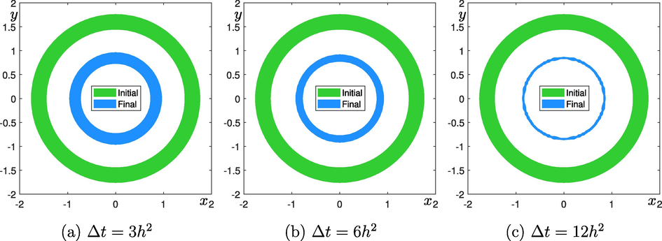
Filled contours of
at levels
and
with respect to
. The green and blue colors are the initial conditions and final results, respectively. Each
is written below each figure.
If we take Eq. (13) as an initial condition, then the continuous solution for the AC equation must be the same as the initial condition as time evolves because it is an equilibrium solution, i.e., for
,
If we plug Eq. (15) into the AC Eq. (1), then the left hand side of the AC equation is zero. The right hand side of the equation becomes
which is also zero. Therefore, we require the numerical solution with an equilibrium solution to have the same property: If we start from an equilibrium numerical initial condition, then we should have the same initial profile as time evolves. However, if we use a relatively large time step in the OSM, then we can see the violation of this property as shown in Fig. 2(a). The circled line denotes the initial profile, Eq. (15). The stared line is the numerical solution after the first step in the OSM, i.e., the solution of the diffusion equation. The squared line is the numerical solution from the nonlinear part in the AC equation. Here, we used
, and
. The nonlinear part dominates the evolution and shows very stiff solution across the interfacial transition layer. Fig. 2 display the results with different time rescaling parameter values of
, and
, respectively. The result with
shows the best among them. The numerical solution shows a similar behavior to that observed in the continuous solution.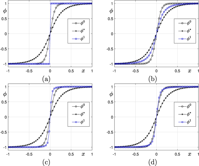
Initial profile (
), the first step (
), and the second step (
) solutions with different r values: (a)
, (b)
, (c)
, and (d)
.
3.2 Effects of optimal time rescaling parameter
Next, we describe the proposed algorithm for computing an optimal r value which makes
be as close as possible to
, where
Fig. 3(a) shows
against the discrete r parameter domain
. Let
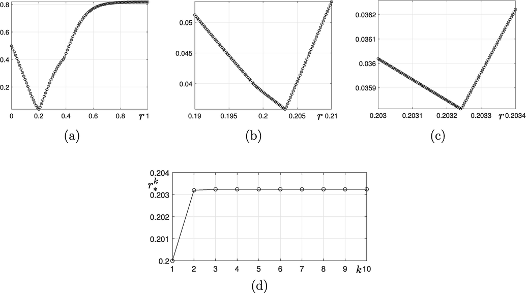
on (a)
, (b)
, and (c)
. (d) is the plot of
against k.
Fig. 3(d) shows the optimal time rescaling parameter values against k. We can confirm these values quickly converge to an optimal value.
We summarize the step by step guide for the proposed algorithm as follows:
Step by step guide for the proposed algorithm
Preprocessing. We compute for some k from Eq. (19).
Using , we compute the next time numerical solution by taking the following two steps:
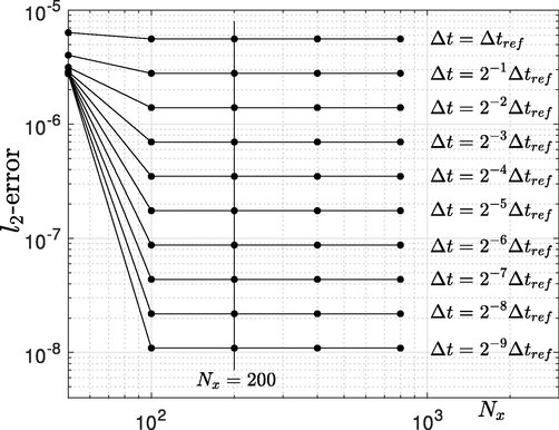
Let
, where a reference time step is defined as
. Fig. 4 shows the optimal time rescaling parameter values
for various m values. We can observe the optimal time rescaling parameter values decreases as we increase m values, i.e., time step sizes. Here, we used
.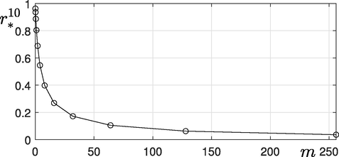
Optimal time rescaling parameter
for various m values.
The optimal time scaling parameter also depends on values. We use and , which is defined in Eq. (14). We have , and for the optimal time rescaling parameter for various values. We can observe that the optimal time scaling parameter values increase as we increase values, i.e., .
3.3 Convergence test
We consider traveling wave solutions of Eq. (1) (Choi et al., 2009):
-errors of the numerical solution for various
.
Let
and we set
with varying
. We define the rate of convergence as
. Table 1 shows that the proposed scheme is first-order accurate in time.
8.00e-4
Rate
4.00e-4
Rate
2.0e-4
Rate
1.0e-4
-error
5.2664e-3
0.95
2.7323e-3
0.97
1.3939e-3
0.98
7.0434e-04
3.4 Comparison between previous and proposed methods
Let us consider an evolution of initially square shape on :
Here, we use
, and
. Fig. 6(a) and (b) display the evolution of the contours of
at zero level with
and
, respectively. Fig. 6(c) and (d) show the contours at levels
and
with
and
, respectively. In the case of
, the result using the standard OSM (Li et al., 2010), we can observe the interfacial transition is not smooth and mosaic, see Fig. 6(a) and (c). However, if we apply the proposed optimal time rescaling parameter
to the nonlinear step, then we have smooth interface profile and uniform transition layer as shown in Fig. 6(b) and (d).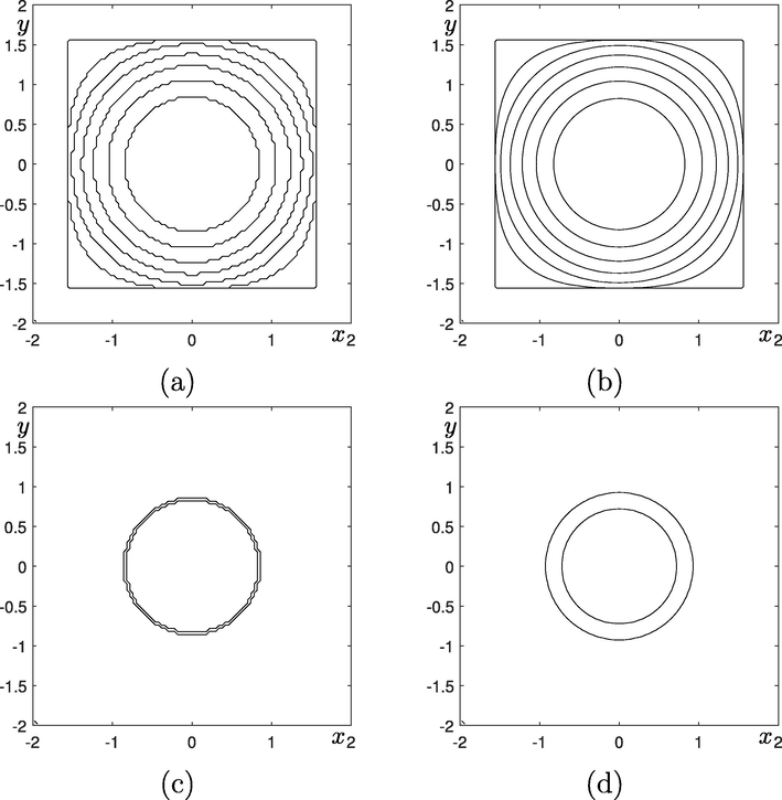
Temporal evolutions of the contours of
at zero level with (a)
and (b)
. Contours at levels
and
with (c)
and (b)
.
Next, let us consider more complex initial profile, which is shown in the first column in Fig. 7(a). Fig. 7(b)–(d) are evolutions of the filled contours of
at zero level with
, and
for the top, middle, and bottom rows, respectively. Here, we use
, and
.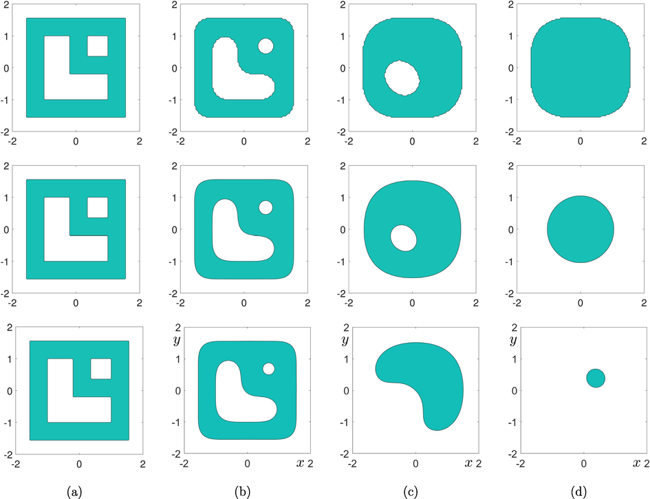
Temporal evolutions of the filled contours of
at zero level with
, and
for the top, middle, and bottom rows, respectively. The times are (a)
, (b)
, (c)
, and (d)
.
In the case of , the result using the standard OSM, we can observe the evolution is delayed because of the domination of the nonlinear effect, see the first row in Fig. 7. However, if we apply the proposed optimal time rescaling parameter to the nonlinear step, then we have smooth and fast evolutions as shown in the second row in Fig. 7. To confirm is optimal parameter value, let us consider a small value of r. The third row in Fig. 7 displays the evolution which is dominated by the diffusion and is far from the motion by mean curvature dynamics.
3.5 Motion by mean curvature
In two-dimensional space, the normal velocity of circular interface satisfies the following geometric law (Jeong and Kim, 2018)
The domain is
. Here, we use
and three different time steps
. The final time
is fixed. We consider
, and
with respect to
, and
, respectively. Fig. 8 shows the computational results with different time steps. It can be confirmed that the analytic and numerical solutions are in good agreement with each other when fine time step is used. However, if we increase the time step, then the difference between the analytic results and numerical results with
becomes larger and larger. The results indicate that
has good performance.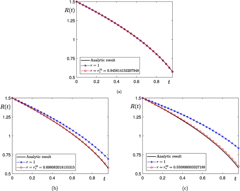
Motion by mean curvature with (a)
, (b)
, and (c)
.
3.6 Application of the proposed method on adaptive mesh
It is not practical to apply phase-field methods using a uniform mesh to real-world problems because of the computational cost. Therefore, it is better to use a non-uniform mesh that is adaptively refined near interfaces. Let us apply the proposed method with an adaptive meshing technique (Jeong et al., 2021), which was recently developed for the AC equation. Let
be the initial condition on
as shown in Fig. 9(a). Fig. 9 shows the snapshots of the interface with adaptive mesh at
, and
from left to right. We can observe the interface evolution according to the motion by mean curvature.
, and
are used. In the case of adaptive mesh computation, we use finite difference method, however, for simplicity of exposition, we use the optimal time rescaling parameter
for
value computed from the Fourier spectral method.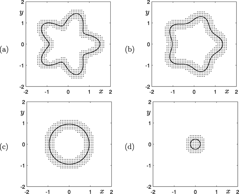
(a), (b), (c), and (d) are the snapshots of the interface with adaptive mesh at
, and
, respectively.
We presented a fast evolution numerical algorithm for the AC equation. One of efficient numerical methods for the AC equation is the OSM. However, if a large time step is used, then the nonlinear part in the OSM dominates the evolution and results in a sharp interfacial transition layer. The evolutions are either mosaic or pinned if a large time step is used. To overcome these problems, a time rescaling method to the nonlinear part of the AC equation was proposed. Computational tests confirmed the performance of the proposed algorithm which makes the evolution fast and interfacial transition layer be uniform. The proposed time step rescaling method can be applied to the other OSM with different spatial discretizations such as FDM and FEM.
Acknowledgment
J. Yang is supported by the National Natural Science Foundation of China (No. 12201657), the China Postdoctoral Science Foundation (No. 2022M713639), and the 2022 International Postdoctoral Exchange Fellowship Program (Talent-Introduction Program) (No. YJ20220221). C. Lee was supported by the National Research Foundation(NRF), Korea, under project BK21 FOUR. The corresponding author (J.S. Kim) was supported by the Brain Korea 21 FOUR from the Ministry of Education of the Republic of Korea. Y. Choi was supported by National Research Foundation of Korea (NRF) grant funded by the Korea government (NRF-2020R1C1C1A0101153712). The authors thank the reviewers for the constructive and helpful comments on the revision of this article.
Declaration of Competing Interest
The authors declare that they have no known competing financial interests or personal relationships that could have appeared to influence the work reported in this paper.
References
- A stabilized bi-grid method for Allen-Cahn equation in finite elements. Comput. Appl. Math.. 2019;38:35.
- [Google Scholar]
- Analytical treatment of two-dimensional fractional Helmholtz equations. J. King. Saud. Univ. -Sci.. 2019;31(4):659-666.
- [Google Scholar]
- An explicit nonstandard finite difference scheme for the Allen-Cahn equation. J. Diff. Equ. Appl.. 2015;21(10):875-886.
- [Google Scholar]
- A microscopic theory for antiphase boundary motion and its application to antiphase domain coarsening. Acta Metall.. 1979;27(6):1085-1095.
- [Google Scholar]
- Comparison of operator splitting schemes for the numerical solution of the Allen-Cahn equation. AIP Adv.. 2019;9(12):125202.
- [Google Scholar]
- Some algorithms for the mean curvature flow under topological changes. Comput. Appl. Math.. 2021;40:104.
- [Google Scholar]
- An unconditionally gradient stable numerical method for solving the Allen-Cahn equation. Phys. A. 2009;338(9):1791-1803.
- [Google Scholar]
- A compact split-step finite difference method for solving the nonlinear Schrödinger equations with constant and variable coefficients. Comput. Phys. Comm.. 2010;181(1):43-51.
- [Google Scholar]
- Analysis of symmetric interior penalty discontinuous Galerkin methods for the Allen-Cahn equation and the mean curvature flow. IMA J. Numer. Anal.. 2015;35(4):1622-1651.
- [Google Scholar]
- RBF collocation approach to calculate numerically the solution of the nonlinear system of qFDEs. J. King Saud. Univ. -Sci.. 2021;33(2):101288.
- [Google Scholar]
- Maximum norm error analysis of an unconditionally stable semi-implicit scheme for multidimensional Allen-Cahn equations. Numer. Methods Partial Differ. Equ.. 2019;35:955-975.
- [Google Scholar]
- Discrete maximum-norm stability of a linearized second-order finite difference scheme for Allen-Cahn equation. Numer. Analys. Appl.. 2017;10:177-183.
- [Google Scholar]
- A new second-order maximum-principle preserving finite difference scheme for Allen-Cahn equations with periodic boundary conditions. Appl. Math. Lett.. 2020;104:106265.
- [Google Scholar]
- Adaptive operator splitting finite element method for Allen-Cahn equation. Numer. Methods Partial Differ. Equ.. 2019;35(3):1290-1300.
- [Google Scholar]
- Analytical and numerical solutions of mathematical biology models: the Newell-Whitehead-Segel and Allen-Cahn equations. Math. Meth. Appl. Sci.. 2020;43(5):2588-2600.
- [Google Scholar]
- An explicit hybrid finite differnece scheme for the Allen-Cahn equation. J. Comput. Appl. Math.. 2018;340:247-255.
- [Google Scholar]
- A practical adaptive grid method for the Allen-Cahn equation. Phys. A. 2021;573:125975.
- [Google Scholar]
- Adaptive linear second-order energy stable schemes for time-fractional Allen-Cahn equation with volume constraint. Commun. Nonlinear Sci. Numer. Simul.. 2020;90:105366.
- [Google Scholar]
- Shape transformation using the modified Allen-Cahn equation. Appl. Math. Lett.. 2020;107:106487.
- [Google Scholar]
- Physical, mathematical, and numerical derivations of the Cahn-Hilliard equation. Comput. Mater. Sci.. 2014;81:216-225.
- [Google Scholar]
- Novel mass-conserving Allen-Cahn equation for the boundedness of an order parameter. Commun. Nonlinear Sci. Numer. Simul.. 2020;85:105224.
- [Google Scholar]
- A semi-analytical Fourier spectral method for the Allen-Cahn equation. Comput. Math. Appl.. 2014;68(3):174-184.
- [Google Scholar]
- A second order operator splitting method for Allen-Cahn type equations with nonlinear source terms. Phys. A. 2015;432(15):24-34.
- [Google Scholar]
- Pinning boundary conditions for phase-field models. Commun. Nonlinear Sci. Numer. Simul.. 2020;82:105060.
- [Google Scholar]
- Effect of space dimensions on equilibrium solutions of Cahn-Hilliard and conservative Allen-Cahn equations. Numer. Math. Theor. Meth. Appl.. 2020;13(3):644-664.
- [Google Scholar]
- An unconditionally energy stable second order finite element method for solving the Allen-Cahn equation. J. Comput. Appl. Math.. 2019;353:38-48.
- [Google Scholar]
- An efficient volume repairing method by using a modified Allen-Cahn equation. Pattern. Recognit.. 2020;107:107478.
- [Google Scholar]
- An unconditionally stable hybrid numerical method for solving the Allen-Cahn equation. Comput. Math. Appl.. 2010;60(6):1591-1606.
- [Google Scholar]
- A reduced-order modified finite difference method preserving unconditional energy-stability for the Allen-Cahn equation. Numer. Methods Partial Differ. Equ.. 2021;37:1869-1885.
- [Google Scholar]
- On Energy Stable, Maximum-Principle Preserving, Second-Order BDF Scheme with Variable Steps for the Allen-Cahn Equation. SIAM J. Numer. Anal.. 2020;58(4):2294-2314.
- [Google Scholar]
- The numerical solution of Cahn-Hilliard (CH) equation in one, two and three-dimensions via globally radial basis functions (GRBFs) and RBFs-differential quadrature (RBFs-DQ) methods. Eng. Anal. Bound. Elem.. 2015;51:74-100.
- [Google Scholar]
- A meshless technique based on generalized moving least squares combined with the second-order semi-implicit backward differential formula for numerically solving time-dependent phase field models on the spheres. Appl. Numer. Math.. 2020;153:248-275.
- [Google Scholar]
- A divergence-free generalized moving least squares approximation with its application. Appl. Numer. Math.. 2021;162:374-404.
- [Google Scholar]
- An asymptotic analysis and numerical simulation of a prostate tumor growth model via the generalized moving least squares approximation combined with semi-implicit time integration. Appl. Math. Model.. 2022;104:826-849.
- [Google Scholar]
- Numerical simulation of a prostate tumor growth model by the RBF-FD scheme and a semi-implicit time discretization. J. Comput. Appl. Math.. 2021;388:113314.
- [Google Scholar]
- Numerical simulation and error estimation of the time-dependent Allen-Cahn equation on surfaces with radial basis functions. J. Sci. Comput.. 2019;79(1):493-516.
- [Google Scholar]
- Exp-function method for some nonlinear PDE’s and a nonlinear ODE’s. J. King. Saud. Univ. -Sci.. 2012;24(1):1-10.
- [Google Scholar]
- Numerical solution for the Kawahara equation using local RBF-FD meshless method. J. King Saud. Univ. -Sci.. 2020;32(4):2277-2283.
- [Google Scholar]
- Experimental and numerical investigation of drop evaporation depending on the shape of the liquid/gas interface. Int. J. Heat Mass Transf.. 2017;105:655-663.
- [Google Scholar]
- Efficient numerical scheme for solving the Allen-Cahn equation. Numer. Methods Partial Differ. Equ.. 2018;34(5):1820-1833.
- [Google Scholar]
- An efficient space-time operator-splitting method for high-dimensional vector-valued Allen-Cahn equations. Int. J. Numer. Method H. 2019;29(9):3437-3453.
- [Google Scholar]
- A fast time two-mesh algorithm for Allen-Cahn equation. Bull. Malays. Math. Sci. Soc.. 2020;43:2417-2441.
- [Google Scholar]
- Stabilized energy factorization approach for Allen-Cahn equation with logarithmic Flory-Huggins potential. J. Sci. Comput.. 2020;82:25.
- [Google Scholar]
- Fast and accurate smoothing method using a modified Allen-Cahn equation. Comput. Aided Des.. 2020;120:102804.
- [Google Scholar]
- Analysis of the operator splitting scheme for the Allen-Cahn equation. Numer. Heat Transfer Part B: Fundam.. 2016;70:472-483.
- [Google Scholar]
- A highly efficient operator-splitting finite element method for 2D/3D nonlinear Allen-Cahn equation. Int. J. Numer. Methods Heat Fluid Flow. 2017;27:530-542.
- [Google Scholar]
- Unconditionally maximum principle preserving finite element schemes for the surface Allen-Cahn type equations. Numer. Methods Partial Differ. Equ.. 2020;36(2):418-438.
- [Google Scholar]
- A reliable numerical method for solving fractional reaction-diffusion equations. J. King Saud. Univ. -Sci.. 2021;33(2):101320.
- [Google Scholar]
- Mathematical modeling and simulation of antibubble dynamics. Numer. Math. Theor. Meth. Appl.. 2020;13(1):81-98.
- [Google Scholar]
- Convergence analysis for the invariant energy quadratization (IEQ) schemes for solving the Cahn-Hilliard and Allen-Cahn equations with general nonlinear potential. J. Sci. Comput.. 2020;82(3):1-28.
- [Google Scholar]
- Fast algorithm for nonlocal Allen-Cahn equation with scalar auxiliary variable approach. Appl. Math. Lett.. 2022;126:107805.
- [Google Scholar]
- Numerical simulation of three dimensional Allen-Cahn equation by high-order compact ADI method. Comput. Phys. Commun.. 2014;185(10):2449-2455.
- [Google Scholar]
Appendix A
Supplementary material
Supplementary data associated with this article can be found, in the online version, at https://doi.org/10.1016/j.jksus.2022.102430.
Supplementary material
The following are the Supplementary data to this article:


