

Translate this page into:
A variable sampling interval one-sided CUSUM control chart for monitoring the multivariate coefficient of variation
⁎Corresponding author. hxl0419@njupt.edu.cn (XueLong Hu),
-
Received: ,
Accepted: ,
This article was originally published by Elsevier and was migrated to Scientific Scholar after the change of Publisher.
Peer review under responsibility of King Saud University.
Abstract
Monitoring techniques based on the multivariate coefficients of variation (MCV) have received a great deal of attention in quality control. Numerous studies have shown that adaptively changing the charting parameters based on the past sample information can improve the performance of a chart in detecting process changes. In view of the performance benefits of adaptive strategies, two one-sided cumulative sum (CUSUM) charts are proposed to monitor the MCV and a variable sampling interval (VSI) strategy is incorporated into these charts. By using the Markov chain method, the formulas for calculating the average and standard deviation of time to signal measures of the VSI CUSUM MCV control charts are derived. Then for the known and unknown shift sizes, the optimization algorithms for obtaining the charting parameters are presented. The superiority of the proposed control charts is confirmed by comparing their performance with two existing MCV charts. Finally, an example using real investment data demonstrates the practical application of the proposed charts.
Keywords
Multivariate Coefficient of Variation
CUSUM
Average Time to Signal
Markov Chain

1 Introduction
Control charts are widely applied as an effective monitoring tool to ensure product quality and production stability in statistical process control (SPC). When there is an assignable cause in an industrial process that can lead to process deterioration or improvement, control charts tend to be triggered with a warning signal indicating the process as out-of-control (OOC). Then, corrective strategies to find and eliminate assignable causes are implemented by practitioners to further ensure the process stability. By preventing anomalies in an early stage, control charts facilitate the reduction of quality costs and thus increase product competitiveness.
Traditionally, the process mean or/and variance is monitored for change detection in a process. Monitoring of the coefficient of variation (CV), which combines the mean and variance in a ratio form, has been much overlooked. In some applications, even though both the mean and the standard deviation have changed, a process may not be OOC when there is a constant ratio between and , see Muhammad et al. (2018). In this case, the CV, denoted by , can be considered as a good monitoring alternative. This can be illustrated in the example of the clinical-chemistry control problem in Kang et al. (2007), in which measurements of chemical characteristics in the patient's blood need to be taken repeatedly. Since the average value of the measurement varies from patient to another, the CV should be monitored instead of the of the process. Hence, the research of CV monitoring is valuable in practical application.
Extensive investigations have been devoted to the performance and enhancement of univariate CV charts. A pioneering study was conducted by Kang et al. (2007), who developed a Shewhart version of the CV chart. Since only the latest sample information was considered, small changes may not be detected by the Shewhart CV chart. Exponentially weighted moving average (EWMA) charts were therefore applied by Castagliola et al. (2011) to deal with scenarios with small and medium changes. Following the same EWMA charting scheme, Zhang et al. (2014) suggested some modifications and further improves its performance in detecting small changes. Instead of using the EWMA scheme, Tran and Tran (2016) applied a cumulative sum (CUSUM) scheme and developed two new one-sided CV charts. More research efforts on CV charts include the run sum CV charts by Teoh et al. (2017), a set of CV charts based on the auxiliary information by Abbasi (2020) among others. A review of univariate CV charts is detailed in Jalilibal et al. (2021).
It can be seen that the aforementioned studies aimed at monitoring one single quality characteristic. However, it is more common that simultaneously monitoring MCV are of interest. For instance, in genetics and biometrics, CV is an important measure of the relative variability of different populations, where usually various characteristics of individuals are involved. Since the correlation exists among these characteristics, univariate CV for different characteristics cannot be taken into account separately, see Albert and Zhang (2010). Similarly, the relative variability of 14 traits in female pouched gophers was measured in Soulé and Zegers (1996), and in this process, the MCV was monitored instead of the univariate CV, which ignores the correlation structure between different variables. Hence, the study and enhancement of MCV charts is a worthy concern in SPC research.
Among the existing studies, Yeong et al. (2016) first designed the MCV chart using the Shewhart scheme. Subsequently, Lim et al. (2017) improved the Shewhart charts by integrating the run sum feature and the proposed chart showed a stronger sensitivity in detecting changes than the Shewhart charts. Another effort to improve the Shewhart MCV charts is the two one-sided synthetic charts suggested by Nguyen et al. (2019a,b). Further, the MCV chart was extended to the EWMA framework for small shift detection by Giner-Bosch et al. (2019). To overcome the limitation that the existing MCV schemes are for sample sizes greater than 1, an EWMA scheme was designed for individual observations in Haq and Khoo (2022). Examples of other research contributions include MCV charts considering measurement errors by Ayyoub et al. (2020), sensitivity of Shewhart MCV charts for short runs by Khatun et al. (2019), and comparison among various MCV charts in Phase I by Abbasi and Adegoke (2018).
The control charts previously discussed follow a fixed chart parameter strategy, i.e., the chart parameters of these charts are always fixed regardless of the previous sample information. Incorporating the adaptive features to the control charts with fixed chart parameters is one of the strategies to improve chart performance. As shown in the comprehensive study of the adaptive charts properties in Epprecht et al. (2003), adaptive control charts outperform their non-adaptive counterparts in shift detection. Readers can see the work in Tagaras (1998) for more research on adaptive control charts.
Both univariate CV and MCV control charts can benefit from integration of adaptive strategies. For instance, the variable sampling interval (VSI) and the variable sample size (VSS) strategies were applied to traditional Shewhart CV chart in order to detect outliers more quickly by Castagliola et al. (2013) and Castagliola et al. (2015), respectively. The VSI feature was also incorporated to the EWMA CV chart by Yeong et al. (2017) and to the CUSUM CV squared chart by Tran and Heuchenne (2021). Yeong et al. (2018) considered the combination of VSI, VSS and variable control limits for CV chart and designed a variable parameters (VP) CV chart. Recently, Yeong et al. (2023) improved the performance of the run sum charts for CV by combining variable sample size and sampling interval (VSSI) and VP. With regard to the adaptive MCV charts, Khaw et al. (2018) favored the use of VSSI MCV chart based on the numerical comparison among the VSI, VSS and VSSI control charts. Chew et al. (2019) designed a VP MCV chart and showed its higher sensitivity than existing MCV charts. Nguyen et al. (2019a,b) increased the detection sensitivity of Shewhart MCV charts by combining VSI features. Haq and Khoo (2019) suggested two adaptive EWMA (AEWMA) charts for monitoring univariate CV and MCV. Focusing on detection of the downward shift in the MCV, Chew and Khaw (2020) designed a one-sided control chart with VSSI features. Nguyen et al. (2021) designed two one-sided EWMA MCV charts with VSI features and further studied the effect of measurement errors on their performance. Sabahno and Celano (2023) designed the Shewhart scheme in the presence of autocorrelation and incorporated VP features to improve its monitoring performance for MCV.
As reviewed above, most researches on adaptive MCV charts are limited to the Shewhart type. The EWMA and CUSUM types, which are more effective in detecting small fluctuations, have received less attention. In traditional monitoring context, CUSUM charts are known to achieve optimal performance for specific shifts and is superior to EWMA charts when actual shifts are as expected, see Hawkins and Wu (2014). Such advantage of CUSUM charts was also validated in the applications of monitoring normal ratio by Tran et al. (2018) and univariate CV by Tran and Tran (2016). In order to enhance adaptive MCV chart in detecting small shifts, this paper combines VSI features with CUSUM MCV charts, and designs two one-sided VSI CUSUM MCV charts based on the one-sided CUSUM MCV charts proposed by Hu et al. (2023). Superiority of the proposed charts is clarified through numerical experiments, where performance criteria including average signal time (ATS) and expected ATS (EATS) are thoroughly evaluated using the Markov chain model under deterministic and unknown shift size conditions.
The structure of this paper is organized as follows. First, we present a simple description of the basic properties of the sample MCV squared in Section 2, where the one-sided VSI EWMA MCV charts and the CUSUM MCV charts are also briefly introduced. In Section 3, the proposed one-sided VSI CUSUM MCV charts are constructed, along with their ATS properties derived from a Markov chain model. To minimize the value of OOC ATS and EATS, an optimization algorithm are presented under deterministic and unknown shift size conditions in Section 3. Numerical studies on performance comparison among the proposed and some benchmark control charts are presented in Section 4. A real case analysis using the proposed charts is illustrated in Section 5. The last Section 6 outlines the main conclusions and future recommendations.
2 Some existing MCV charts
First, the basic properties of the sample MCV squared are briefly reviewed. Then, some existing MCV charts are introduced, including the one-sided VSI EWMA MCV charts and the CUSUM MCV charts.
2.1 Basic properties of the sample MCV squared
Denote by
a random sample of size
. Each
is a p-dimensional vector from a multivariate normal distribution with mean parameter
and covariance parameter
, i.e.,
,
. The population MCV is then derived as
Then the sample MCV is
To monitor the MCV, the distribution of the MCV
or the MCV squared (
) is of interest. It has been derived that the cumulative distribution function (c.d.f.) of
is
2.2 The existing one-sided VSI EWMA MCV charts
Considering that the Shewhart chart focuses only on the latest sample information, a one-sided MCV chart based on the EWMA scheme was proposed in Giner-Bosch et al. (2019). The VSI feature is then incorporated by Ayyoub et al. (2022) to further enhance the EWMA MCV chart.. In both studies, only upward shifts were considered, while downward shifts were neglected. Motivated by this, Nguyen et al. (2021) suggested two one-sided VSI EWMA MCV charts with a “restart state” to overcome the “inertia problem” in the previous VSI EWMA scheme. The construction methods of their charts are described as follows.
The charting statistic for the upward EWMA MCV chart is
Furthermore, the upper warning limit (UWL) and lower warning limit (LWL) are defined in Nguyen et al. (2021) as
2.3 The existing one-sided CUSUM MCV charts
To make use of the advantage of the CUSUM control chart in detecting small shifts in univariate CV, Hu et al. (2023) have suggested two one-sided MCV charts based on the CUSUM scheme. The charting methods are as follows.
The charting statistic for the upward CUSUM chart is
The charting statistic for the downward CUSUM chart is
3 The proposed one-sided VSI CUSUM MCV charts
The construction, performance measures and optimal design procedures of the VSI CUSUM MCV control charts are provided in this section. First, Section 3.1 combines the VSI strategy with the standard CUSUM MCV charts and describes in detail the construction of the VSI CUSUM MCV control charts. Second, the performance metrics are derived based on a Markov chain method in Section 3.2. Finally, optimization algorithms for calculating control limits by minimizing the performance metrics are presented.
3.1 The proposed one-sided VSI CUSUM MCV charts
The above CUSUM MCV charts proposed in Hu et al. (2023) belongs to the non-adaptive type charts, which adopt a fixed sampling interval (FSI) strategy. To be consistent with the VSI EWMA MCV charts reviewed in Section 2.2, the VSI CUSUM MCV control charts are constructed by adapting the fixed sampling interval in the original FSI chart into the variable version
, while the UCL and the LCL remains the same. The VSI
of the proposed VSI CUSUM MCV control charts changes at both
and
levels for different values of the current statistic
or
, where
. To implement the VSI CUSUM MCV chart, it is necessary to introduce new warning limits (UWL and LWL), which are defined as follows:
-
When the monitored statistic or falls into the safe region, the process is declared as IC and a long sampling interval is adopted to draw the next sample.
-
When the monitored statistic or falls into the warning region, the process is IC but with a high risk of being OOC. Hence, the next sample interval it set to be short, say , to detect potential assignable causes more quickly.
-
When the monitored statistic or falls into the OOC region, the process is declared as OOC and prompt actions should be taken to locate and remove assignable causes quickly.
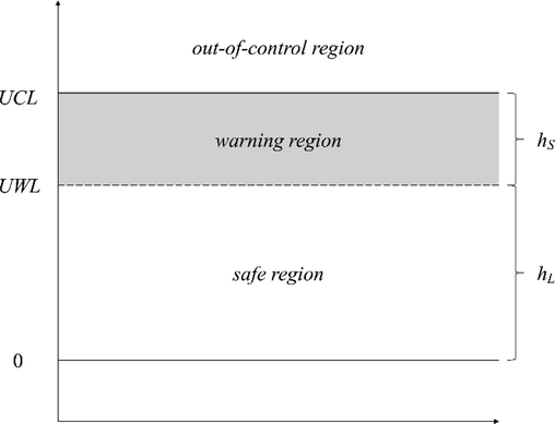
- The region division of the upward VSI CUSUM MCV control chart.
3.2 Performance measures
Traditionally, in order to evaluate the performance of FSI type charts, criteria based on the run length distribution is widely used. Among these criteria, the average run length (ARL) is the most commonly adopted. For VSI type charts, the time between two successive samples varies. Therefore, ARL is not applicable. To evaluate the properties of VSI type control charts,. the ATS and standard deviation of time to signal (SDTS) are suggested. ATS indicates the expected time to the appearance of an OOC signal since the process monitoring is started, and SDTS measures the variability of the time to signal. A well-performed control chart is expected to falsely alarm at a low rate for an IC process and to trigger a signal as fast as possible for an OOC process. Therefore, a large IC ATS ( ) and a small OOC ATS ( ) are considered to be the indication of excellent chart performance.
For FSI type charts, the ATS is represented as
For VSI type charts, the ATS is computed as
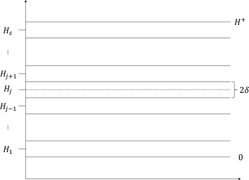
Sub-division of the IC range.
By definition, , , denotes the midpoint of the subinterval . The width of each subinterval is and decreases with since . When is sufficiently large, the subinterval becomes so narrow that all the values in the subinterval can be approximated as . When indicates the proposed charts to “restart”. The transition probability from state to state is provided as follows.
-
For the upward chart,
-
For the downward chart,
From Eqs. (17) and (21), the expected sampling interval
is obtained as:
The denominator in Eq. (23) is the formula for ARL as in Brook and Evans (1972). To make fair comparison, the same IC values of and are imposed for both FSI and VSI types of charts. Then, the OOC metrics and are evaluated for the comparison purpose. Without the loss of generality, we assumed that time unit, which leads to by plugging into Eq. (16).
3.3 Optimization algorithm
This section provides an optimization algorithm for minimizing and of the VSI CUSUM MCV charts. For the known shift size case, Section 3.3.1 presents an optimization model to determine the chart parameters that minimizes the of the proposed control charts. For the unknown shift size case, the EATS measure is proposed and the corresponding optimization program is designed in Section 3.3.2.
3.3.1 The known shift size case
Assume the IC is shifted to due to assignable causes. Here is a prespecified shift size. The optimal parameters of VSI CUSUM MCV can be obtained using the optimization algorithm that minimizes the with a given . As proposed in Castagliola et al. (2013), is usually chosen as a fixed couple in the VSI setting. It is acceptable to set a fixed value in advance because in the industrial production process, a certain time interval always exists between the production process of two products or two batches of products. However, predetermining the value of is dubious, since the sampling interval before the next sampling can be arbitrarily chosen when the value of the current statistic falls into the safety region, as long as the chart performance is not affected. For this reason, we propose to predetermine the value of warning limit coefficient instead of . Then we minimize the with respect to (upward chart) or (downward chart) using some small values of . Furthermore, the optimal combination or for the proposed VSI CUSUM MCV charts with a given shift size is calculated as follows.
-
For the chart to detect downward shifts,
subject to the constraint
-
For the chart to detect upward shifts,
subject to the constraint
3.3.2 The unknown shift size case
The optimization model for the VSI CUSUM MCV control charts presented in Section 3.3.1 was designed with the shift size
being predetermined. In the actual production process, however, relevant historical data are hardly possible to be available for predetermining the exact shift size
. In such a situation, according to the work of Tran and Heuchenne (2021), we can use EATS as the performance criterion. Given the range of shift size
, the EATS is computed as
-
for the downward chart,
subject to the constraint
-
for the upward chart,
subject to the constraint
4 Numerical results and comparison
Through numerical experiments, we intend to evaluate the optimal performance of the proposed VSI CUSUM MCV control charts. Moreover, comparison is conducted among the VSI CUSUM MCV, the FSI CUSUM MCV charts proposed by Hu et al. (2023), and the VSI EWMA MCV charts proposed by Nguyen et al. (2021). Cases of both known and unknown shift sizes are explored. Without loss of generality, the is set to 370.4 and . In this paper, we set to ensure that the sampling interval is a suitable minimum so that a sufficient number of samples can be acquired. In addition, it should be noted that setting is impractical, see Aparisi and Haro (2001).
4.1 Optimal triples of the VSI CUSUM MCV charts
The optimal triples when , and when are presented in the Table 1 for , , and . For the sake of brevity, similar tables for are presented in Table A1–A3 in the supplementary material. From these tables, the following conclusions are drawn.
-
In general, given , , and , the values of and vary with . Specifically, decrease and , increase as decreases. Considering the setting , , and , the optimal triples for the VSI CUSUM MCV control chart are if and these values change to if (Table 1).
-
In general, given , , and , the values of and vary with . Specifically, the values of and increase and the values of decrease as decreases. In the case that , , and , the optimal triples for the VSI CUSUM MCV control chart are if and these values change to if (Table 1).
-
In general, given , , and , the values of and vary with . Specifically, the values of and decrease and the values of increase as decreases. For instance, when , , and , the optimal triples for the VSI CUSUM MCV control chart are if and these values are if (Table 1 and Table A1 in the supplementary material).
-
In general, given , , and , the values of and vary with . Specifically, the values of and decrease and the values of increase as increases. For instance, when , , and , the optimal triples for the VSI CUSUM MCV control chart are if and if .
-
In general, given , , and , the IC has a slight effect on the values of and . For instance, when , , and , the optimal triples for the VSI CUSUM MCV control chart are if and if . That is, an increase of leads to a slight increase in and and a slight decrease in .
| 0.1 | 0.5 | (1.010,0.856,1.12) | (0.700,1.805,1.11) | (0.535,2.667,1.13) | (1.264,0.702,1.05) | (0.885,1.437,1.05) | (0.675,2.182,1.07) |
| 0.75 | (0.497,2.932,1.71) | (0.406,3.693,1.46) | (0.380,3.956,1.32) | (0.632,2.385,1.46) | (0.495,3.201,1.32) | (0.431,3.711,1.26) | |
| 0.9 | (0.197,6.915,3.44) | (0.183,7.273,2.50) | (0.169,7.660,2.18) | (0.251,5.973,2.83) | (0.224,6.488,2.15) | (0.210,6.793,1.89) | |
| 1.1 | (0.191,8.588,2.83) | (0.176,8.911,2.24) | (0.162,9.231,2.05) | (0.241,7.516,2.46) | (0.222,7.829,1.99) | (0.213,8.001,1.81) | |
| 1.25 | (0.457,5.486,1.66) | (0.406,5.854,1.47) | (0.353,6.316,1.43) | (0.584,4.536,1.49) | (0.480,5.107,1.37) | (0.441,5.374,1.31) | |
| 1.5 | (0.872,3.773,1.25) | (0.726,4.211,1.19) | (0.662,4.445,1.16) | (1.104,2.986,1.16) | (0.884,3.478,1.13) | (0.801,3.711,1.11) | |
| 0.2 | 0.5 | (0.984,0.851,1.13) | (0.675,1.833,1.11) | (0.540,2.553,1.12) | (1.194,0.747,1.07) | (0.846,1.491,1.06) | (0.660,2.182,1.07) |
| 0.75 | (0.487,2.915,1.73) | (0.398,3.693,1.47) | (0.380,3.871,1.31) | (0.619,2.381,1.48) | (0.486,3.201,1.33) | (0.432,3.637,1.26) | |
| 0.9 | (0.193,6.925,3.51) | (0.180,7.275,2.53) | (0.166,7.660,2.20) | (0.246,6.003,2.89) | (0.221,6.487,2.17) | (0.207,6.793,1.91) | |
| 1.1 | (0.184,8.776,2.86) | (0.170,9.098,2.25) | (0.164,9.232,2.02) | (0.233,7.701,2.49) | (0.215,8.013,2.00) | (0.196,8.373,1.87) | |
| 1.25 | (0.438,5.714,1.71) | (0.380,6.155,1.51) | (0.362,6.317,1.41) | (0.562,4.731,1.51) | (0.494,5.107,1.36) | (0.452,5.373,1.30) | |
| 1.5 | (0.834,4.001,1.27) | (0.716,4.364,1.20) | (0.633,4.676,1.17) | (1.063,3.171,1.17) | (0.883,3.582,1.13) | (0.754,3.956,1.12) | |
| 0.3 | 0.5 | (0.944,0.836,1.13) | (0.621,1.952,1.14) | (0.490,2.748,1.15) | (1.145,0.736,1.07) | (0.801,1.529,1.07) | (0.630,2.209,1.08) |
| 0.75 | (0.472,2.882,1.76) | (0.383,3.693,1.49) | (0.367,3.871,1.32) | (0.599,2.372,1.50) | (0.470,3.201,1.34) | (0.410,3.711,1.28) | |
| 0.9 | (0.188,6.928,3.62) | (0.175,7.275,2.58) | (0.162,7.660,2.22) | (0.238,6.041,2.98) | (0.200,6.858,2.33) | (0.203,6.793,1.93) | |
| 1.1 | (0.174,9.092,2.90) | (0.153,9.601,2.36) | (0.148,9.730,2.10) | (0.220,8.002,2.60) | (0.204,8.291,2.06) | (0.198,8.407,1.85) | |
| 1.25 | (0.417,6.028,1.73) | (0.360,6.487,1.53) | (0.328,6.793,1.46) | (0.529,5.048,1.55) | (0.469,5.393,1.38) | (0.423,5.714,1.33) | |
| 1.5 | (0.776,4.381,1.29) | (0.673,4.720,1.22) | (0.618,4.932,1.18) | (0.990,3.498,1.19) | (0.840,3.865,1.14) | (0.719,4.236,1.14) | |
| 0.5 | 0.5 | (0.820,0.784,1.16) | (0.516,2.052,1.17) | (0.460,2.449,1.12) | (0.981,0.748,1.10) | (0.699,1.549,1.08) | (0.500,2.590,1.13) |
| 0.75 | (0.427,2.723,1.87) | (0.353,3.479,1.49) | (0.315,3.956,1.37) | (0.536,2.353,1.59) | (0.432,3.117,1.36) | (0.385,3.564,1.27) | |
| 0.9 | (0.174,6.789,3.98) | (0.158,7.273,2.75) | (0.147,7.660,2.32) | (0.218,6.090,3.26) | (0.201,6.488,2.31) | (0.189,6.793,1.99) | |
| 1.1 | (0.142,10.116,3.03) | (0.130,10.438,2.41) | (0.128,10.500,2.12) | (0.187,8.886,2.73) | (0.173,9.189,2.15) | (0.168,9.296,1.94) | |
| 1.25 | (0.339,7.171,1.83) | (0.308,7.462,1.58) | (0.289,7.661,1.49) | (0.444,6.003,1.66) | (0.377,6.487,1.49) | (0.341,6.793,1.42) | |
| 1.5 | (0.623,5.570,1.37) | (0.548,5.874,1.27) | (0.500,6.102,1.24) | (0.819,4.471,1.27) | (0.679,4.898,1.21) | (0.632,5.071,1.17) | |
4.2 OOC performance of the VSI CUSUM MCV charts
Table 2 presents the values of the three competing charts for , , , and . For the sake of brevity, similar tables for are presented in Tables B1–B3 in the supplementary material. Conclusions are presented as follows (the SDRL values are also commented on in the paper even if they are not shown in these tables):
-
Given the values of , , and , performance of the VSI CUSUM MCV charts is largely influenced by the sample size . For instance, when , , and , the values of the upward VSI CUSUM MCV chart for are (16.68, 13.45) and (11.58, 8.95), respectively (see Table 2).
-
Given the values of , , and , an increase in the value of the IC negatively impact the performance of the VSI CUSUM MCV charts. For instance, with , , and , the value of the VSI CUSUM MCV chart increases from 16.68 to 17.35 when the value of increases from 0.1 up to 0.2 (see Table 2).
-
Given the values of , , and , the detection efficiency of the VSI CUSUM MCV charts is enhanced when the dimension has an increasing trend. In the scenario that , , and , we have and if , and we have and if (see Table 2 and Table B1 in the supplementary material).
-
Given the values of , , and , the warning limit coefficient slightly affected the OOC performance of the VSI CUSUM MCV charts. For instance, when , , and , we have and if , and we have and if (see Table 2).
| 0.1 | 0.5 | 2.43 | (1.36,2.31) | (1.50,1.66) | (1.73,1.47) | 1.62 | (1.15,2.03) | (1.22,1.48) | (1.29,1.29) |
| 0.75 | 8.29 | (3.48,4.17) | (3.77,3.78) | (4.11,4.21) | 5.63 | (2.52,3.21) | (2.72,2.71) | (2.96,2.83) | |
| 0.9 | 32.67 | (14.93,15.56) | (15.46,17.43) | (16.03,19.70) | 23.36 | (10.31,10.94) | (10.72,11.81) | (11.18,13.27) | |
| 1.1 | 32.07 | (16.68,17.18) | (17.01,18.59) | (17.34,20.58) | 23.26 | (11.58,12.08) | (11.85,12.75) | (12.13,14.05) | |
| 1.25 | 8.99 | (4.64,5.06) | (4.75,4.87) | (4.87,5.13) | 6.27 | (3.30,3.72) | (3.39,3.45) | (3.48,3.55) | |
| 1.5 | 3.37 | (2.10,3.45) | (2.13,2.20) | (2.18,2.17) | 2.37 | (1.62,2.03) | (1.64,1.74) | (1.67,1.67) | |
| 0.2 | 0.5 | 2.47 | (1.37,2.33) | (1.53,1.67) | (1.79,1.48) | 1.65 | (1.16,2.05) | (1.23,1.48) | (1.32,1.30) |
| 0.75 | 8.51 | (3.57,4.26) | (3.87,3.89) | (4.23,4.35) | 5.78 | (2.58,3.28) | (2.79,2.77) | (3.05,2.92) | |
| 0.9 | 33.56 | (15.41,16.07) | (15.95,17.99) | (16.54,20.34) | 24.09 | (10.66,11.32) | (11.09,12.24) | (11.56,13.82) | |
| 1.1 | 33.23 | (17.35,17.84) | (17.71,19.41) | (18.05,21.46) | 24.21 | (12.08,12.58) | (12.38,13.39) | (12.65,14.73) | |
| 1.25 | 9.43 | (4.84,5.25) | (4.96,5.09) | (5.09,5.39) | 6.60 | (3.45,3.88) | (3.54,3.60) | (3.64,3.72) | |
| 1.5 | 3.58 | (2.19,3.56) | (2.23,2.28) | (2.27,2.26) | 2.52 | (1.68,2.08) | (1.70,1.80) | (1.74,1.73) | |
| 0.3 | 0.5 | 2.53 | (1.39,2.39) | (1.58,1.69) | (1.88,1.49) | 1.70 | (1.18,2.09) | (1.25,1.50) | (1.37,1.30) |
| 0.75 | 8.86 | (3.71,4.43) | (4.03,4.07) | (4.43,4.58) | 6.05 | (2.68,3.41) | (2.90,2.89) | (3.19,3.08) | |
| 0.9 | 35.04 | (16.21,16.93) | (16.78,19.00) | (17.40,21.50) | 25.28 | (11.26,11.92) | (11.72,12.97) | (12.21,14.65) | |
| 1.1 | 35.23 | (18.50,18.97) | (18.88,20.76) | (19.23,23.01) | 25.81 | (12.92,13.40) | (13.24,14.30) | (13.55,15.80) | |
| 1.25 | 10.20 | (5.19,5.59) | (5.32,5.48) | (5.46,5.83) | 7.17 | (3.69,4.11) | (3.80,3.86) | (3.90,4.02) | |
| 1.5 | 3.94 | (2.34,2.70) | (2.39,2.43) | (2.44,2.43) | 2.77 | (1.79,2.16) | (1.81,1.89) | (1.85,1.84) | |
| 0.5 | 0.5 | 2.73 | (1.46,2.53) | (1.77,1.72) | (2.29,1.57) | 1.86 | (1.23,2.20) | (1.33,1.54) | (1.57,1.32) |
| 0.75 | 9.98 | (4.16,5.00) | (4.60,4.69) | (5.12,5.39) | 6.87 | (3.00,3.77) | (3.29,3.26) | (3.66,3.59) | |
| 0.9 | 39.77 | (18.91,19.81) | (19.55,22.37) | (20.33,25.37) | 29.01 | (13.20,14.01) | (13.71,15.45) | (14.30,17.43) | |
| 1.1 | 42.35 | (22.48,22.90) | (22.99,25.71) | (23.47,28.67) | 31.12 | (15.74,16.17) | (16.17,17.68) | (16.52,19.62) | |
| 1.25 | 12.99 | (6.41,6.76) | (6.62,6.86) | (6.79,7.40) | 9.10 | (4.52,4.90) | (4.66,4.75) | (4.79,5.05) | |
| 1.5 | 5.22 | (2.87,3.17) | (2.94,2.96) | (3.01,3.03) | 3.63 | (2.13,2.46) | (2.18,2.21) | (2.23,2.20) | |
4.3 Comparisons with some existing MCV control charts
Control charts for comparison include the VSI CUSUM MCV charts, the corresponding FSI CUSUM MCV control charts proposed by Hu et al. (2023) and VSI EWMA MCV charts designed by Nguyen et al. (2021). The results from numerical experiments show the superiority of the VSI CUSUM MCV charts over the competing ones.
4.3.1 The known shift size case
The analysis of Table 2 and Tables B1–B3 in the supplementary material shows that whatever the values of , , and are, the values of the VSI CUSUM MCV charts are smaller than those corresponding to the FSI CUSUM MCV charts. Taking the downward CUSUM MCV chart as an example, in Table B2 in the supplementary material, when , , and , the optimal value of the FSI chart is 39.54 for , which is almost two times of the of the VSI counterpart. Similarly, considering the upward CUSUM MCV chart, when the shift is increased to , the optimal value of the VSI chart is . This is also much smaller than the for the corresponding FSI type chart. This fact clearly demonstrates that the detection efficiency of the standard CUSUM scheme for the MCV is remarkably enhanced by incorporating the VSI strategy.
The values presented in Table 2 and Tables B1–B3 in the supplementary material show the advantage of the VSI CUSUM MCV charts over VSI EWMA MCV charts designed by Nguyen et al. (2021). When , the VSI CUSUM MCV charts have better detection performance. For instance, in Table B3 in the supplementary material, when , , and , the values of the downward VSI CUSUM MCV chart and VSI EWMA MCV chart are 5.01 and 5.70 for . When , the performance comparison of these two charts has a great difference for different values of the . When the value of is small, the VSI CUSUM MCV charts still outperform the VSI EWMA MCV charts. As shown in Table B3 in the supplementary material, when , , , and , we have for the downward VSI CUSUM MCV chart and for the downward VSI EWMA MCV chart. However, when the value of is large, VSI EWMA MCV charts have a slight advantage against the VSI CUSUM MCV charts. For instance, for the same case studied above but with , the of the downward VSI EWMA MCV chart is smaller than the of the downward VSI CUSUM MCV chart.
In summary, the detection ability of the VSI CUCUM MCV control charts outperform their FSI counterparts across the board for all shifts and show superiority over the VSI EWMA MCV charts in almost all cases except when the warning limit coefficient and the shift size are simultaneously large.
4.3.2 The unknown shift size case
The OOC EATS
is adopted to compare different MCV charts over a shift range with the shift
assumed to be uniformly distributed. Following Eqs. (27) and (28), Table 3 shows the optimal triples
and
of the proposed charts corresponding to
and
respectively. Other settings are
,
,
and
. The corresponding values of the
are listed in Table 4. In the scenario
,
,
and
, the optimal parameters
of the downward VSI CUSUM MCV chart are calculated as
by minimizing the
over the shift range
in Table 3. The optimal
is then obtained as
. In addition, the
values of the VSI EWMA MCV charts and the FSI CUSUM MCV charts are also presented in Table 4 for the comparison purpose. For instance, with the same parameter settings, the optimal
values of the downward VSI EWMA MCV chart and FSI CUAUM MCV chart are
and
, respectively.
0.10
(0.158,7.992,4.00)
(0.136,8.705,2.98)
(0.122,9.232,2.67)
(0.179,7.551,3.57)
(0.154,8.275,2.70)
(0.148,8.465,2.34)
(0.222,7.999,2.52)
(0.177,8.887,2.19)
(0.162,9.230,2.01)
(0.236,7.594,2.49)
(0.199,8.275,2.08)
(0.176,8.756,1.95)
0.20
(0.157,7.941,4.04)
(0.136,8.649,3.00)
(0.121,9.232,2.69)
(0.178,7.528,3.61)
(0.152,8.275,2.72)
(0.137,8.781,2.47)
(0.207,8.330,2.67)
(0.170,9.104,2.25)
(0.159,9.359,2.04)
(0.230,7.746,2.50)
(0.187,8.557,2.16)
(0.177,8.778,1.94)
0.30
(0.156,7.842,4.11)
(0.136,8.537,3.03)
(0.129,8.781,2.58)
(0.176,7.475,3.67)
(0.149,8.272,2.76)
(0.146,8.372,2.37)
(0.197,8.607,2.70)
(0.163,9.347,2.25)
(0.153,9.587,2.04)
(0.221,7.996,2.53)
(0.180,8.781,2.17)
(0.169,9.047,1.98)
0.50
(0.155,7.361,4.31)
(0.130,8.277,3.18)
(0.128,8.372,2.56)
(0.172,7.238,3.86)
(0.146,8.045,2.85)
(0.137,8.373,2.46)
(0.166,9.541,2.77)
(0.141,10.149,2.28)
(0.134,10.330,2.09)
(0.196,8.710,2.66)
(0.161,9.449,2.21)
(0.152,9.685,2.01)
0.10
(0.156,8.000,4.07)
(0.130,8.892,3.17)
(0.121,9.231,2.69)
(0.175,7.628,3.64)
(0.148,8.432,2.83)
(0.138,8.781,2.46)
(0.224,7.999,2.49)
(0.168,9.114,2.26)
(0.158,9.367,2.06)
(0.231,7.702,2.51)
(0.200,8.276,2.07)
(0.176,8.778,1.95)
0.20
(0.154,7.997,4.13)
(0.128,8.891,3.20)
(0.131,8.782,2.56)
(0.174,7.604,3.68)
(0.147,8.410,2.85)
(0.136,8.781,2.48)
(0.200,8.491,2.70)
(0.165,9.244,2.26)
(0.155,9.488,2.05)
(0.225,7.847,2.53)
(0.184,8.648,2.17)
(0.172,8.924,1.99)
0.30
(0.151,7.971,4.24)
(0.132,8.622,3.08)
(0.128,8.782,2.59)
(0.172,7.559,3.74)
(0.149,8.276,2.77)
(0.145,8.398,2.38)
(0.191,8.749,2.73)
(0.159,9.467,2.26)
(0.148,9.730,2.09)
(0.221,7.999,2.52)
(0.177,8.860,2.18)
(0.166,9.119,1.99)
0.50
(0.149,7.553,4.44)
(0.130,8.277,3.19)
(0.117,8.781,2.71)
(0.168,7.355,3.93)
(0.144,8.136,2.88)
(0.137,8.373,2.46)
(0.163,9.585,2.80)
(0.139,10.174,2.29)
(0.132,10.349,2.10)
(0.193,8.756,2.68)
(0.159,9.481,2.22)
(0.149,9.731,2.06)
0.10
(0.154,7.999,4.14)
(0.129,8.890,3.21)
(0.120,9.231,2.72)
(0.171,7.712,3.71)
(0.145,8.506,2.86)
(0.137,8.782,2.47)
(0.197,8.543,2.73)
(0.163,9.291,2.27)
(0.153,9.532,2.06)
(0.226,7.823,2.54)
(0.184,8.630,2.18)
(0.172,8.909,2.00)
0.20
(0.152,7.998,4.21)
(0.127,8.890,3.24)
(0.119,9.232,2.74)
(0.170,7.696,3.75)
(0.144,8.486,2.88)
(0.136,8.781,2.49)
(0.193,8.686,2.74)
(0.160,9.413,2.27)
(0.151,9.646,2.06)
(0.220,7.964,2.55)
(0.180,8.754,2.18)
(0.169,9.020,2.00)
0.30
(0.149,7.997,4.32)
(0.125,8.890,3.30)
(0.116,9.231,2.77)
(0.168,7.662,3.82)
(0.143,8.439,2.91)
(0.143,8.449,2.40)
(0.185,8.925,2.76)
(0.155,9.597,2.26)
(0.147,9.810,2.09)
(0.223,8.000,2.51)
(0.177,8.888,2.17)
(0.164,9.207,2.00)
0.50
(0.144,7.785,4.60)
(0.129,8.328,3.21)
(0.118,8.781,2.71)
(0.164,7.487,4.00)
(0.140,8.276,3.00)
(0.137,8.373,2.46)
(0.160,9.700,2.83)
(0.137,10.271,2.31)
(0.130,10.439,2.11)
(0.190,8.829,2.71)
(0.158,9.543,2.24)
(0.150,9.735,2.06)
0.10
(0.151,7.999,4.26)
(0.125,8.938,3.28)
(0.107,9.730,2.93)
(0.167,7.800,3.79)
(0.142,8.572,2.90)
(0.136,8.781,2.49)
(0.189,8.770,2.76)
(0.157,9.487,2.28)
(0.148,9.731,2.11)
(0.220,7.947,2.56)
(0.180,8.741,2.19)
(0.168,9.009,2.00)
0.20
(0.150,7.999,4.32)
(0.125,8.896,3.30)
(0.105,9.730,2.95)
(0.166,7.789,3.84)
(0.142,8.550,2.92)
(0.141,8.556,2.40)
(0.185,8.901,2.77)
(0.154,9.599,2.28)
(0.147,9.788,2.10)
(0.219,7.999,2.55)
(0.176,8.856,2.19)
(0.165,9.115,2.00)
0.30
(0.147,7.999,4.43)
(0.123,8.892,3.35)
(0.115,9.231,2.80)
(0.164,7.759,3.90)
(0.141,8.510,2.95)
(0.141,8.491,2.42)
(0.178,9.121,2.79)
(0.151,9.743,2.32)
(0.142,9.967,2.09)
(0.224,7.999,2.49)
(0.178,8.886,2.16)
(0.163,9.230,1.99)
0.50
(0.136,7.992,4.80)
(0.115,8.889,3.52)
(0.107,9.231,2.89)
(0.160,7.609,4.09)
(0.138,8.327,3.03)
(0.137,8.374,2.47)
(0.155,9.806,2.86)
(0.133,10.353,2.32)
(0.128,10.516,2.12)
(0.187,8.893,2.73)
(0.155,9.592,2.25)
(0.148,9.779,2.07)
0.1
26.62
(16.39,17.27)
(16.06,18.04)
(16.20,19.47)
20.75
(12.83,13.69)
(12.43,13.90)
(12.47,14.87)
14.03
(9.95,10.65)
(9.68,10.06)
(9.64,10.54)
10.96
(7.88,8.68)
(7.58,7.80)
(7.52,8.12)
0.2
27.17
(16.75,17.65)
(16.42,18.44)
(16.58,19.94)
21.24
(13.14,14.02)
(12.73,14.29)
(12.78,15.27)
14.45
(10.24,10.90)
(9.96,10.36)
(9.92,10.87)
11.3
(8.10,8.88)
(7.81,8.04)
(7.75,8.39)
0.3
28.06
(17.35,18.29)
(17.01,19.14)
(17.21,20.68)
22.02
(13.65,14.56)
(13.24,14.90)
(13.31,15.94)
15.16
(10.68,11.33)
(10.42,10.88)
(10.39,11.44)
11.88
(8.45,9.22)
(8.18,8.46)
(8.12,8.84)
0.5
30.81
(19.24,20.28)
(18.92,21.40)
(19.28,23.10)
24.39
(15.22,16.23)
(14.80,16.68)
(14.94,17.95)
17.7
(12.20,12.81)
(12.02,12.73)
(12.03,13.46)
13.81
(9.64,10.32)
(9.38,9.81)
(9.36,10.33)
0.1
28.46
(17.53,18.41)
(17.22,19.35)
(17.40,20.91)
21.64
(13.36,14.23)
(12.97,14.56)
(13.02,15.57)
15.01
(10.63,11.31)
(10.36,10.79)
(10.32,11.32)
11.42
(8.19,8.98)
(7.90,8.13)
(7.83,8.48)
0.2
29.03
(17.91,18.82)
(17.60,19.79)
(17.82,21.39)
22.14
(13.68,14.56)
(13.29,14.94)
(13.35,15.97)
15.45
(10.92,11.58)
(10.65,11.12)
(10.63,11.67)
11.79
(8.41,9.19)
(8.13,8.39)
(8.07,8.76)
0.3
29.97
(18.54,19.49)
(18.24,20.53)
(18.48,22.18)
22.95
(14.21,15.12)
(13.81,15.53)
(13.90,16.65)
16.22
(11.40,12.05)
(11.15,11.68)
(11.14,12.28)
12.4
(8.78,9.49)
(8.51,8.83)
(8.47,9.24)
0.5
32.86
(20.54,21.57)
(20.26,22.92)
(20.66,24.72)
25.4
(15.85,16.82)
(15.44,17.39)
(15.60,18.73)
18.97
(13.05,13.67)
(12.88,13.67)
(12.90,14.46)
14.43
(10.04,10.66)
(9.78,10.26)
(9.77,10.81)
0.1
30.73
(18.94,19.83)
(18.65,20.99)
(18.89,22.68)
22.64
(13.97,14.83)
(13.58,15.26)
(13.65,16.33)
16.2
(11.47,12.13)
(11.20,11.69)
(11.18,12.28)
11.95
(8.54,9.32)
(8.25,8.51)
(8.19,8.89)
0.2
31.32
(19.34,20.19)
(19.06,21.48)
(19.32,23.18)
23.15
(14.30,15.18)
(13.92,15.65)
(13.99,16.75)
16.69
(11.78,12.44)
(11.52,12.05)
(11.51,12.67)
12.33
(8.77,9.55)
(8.49,8.79)
(8.44,9.19)
0.3
32.31
(20.01,20.88)
(19.74,22.24)
(20.03,24.06)
23.98
(14.85,15.76)
(14.46,16.26)
(14.58,17.45)
17.53
(12.31,12.96)
(12.07,12.67)
(12.07,13.34)
12.98
(9.17,9.93)
(8.90,9.25)
(8.86,9.69)
0.5
35.37
(22.15,23.17)
(21.92,24.79)
(22.36,26.72)
26.53
(16.55,17.51)
(16.16,18.19)
(16.35,19.61)
20.52
(14.11,14.74)
(13.96,14.83)
(13.99,15.68)
15.13
(10.49,11.12)
(10.24,10.76)
(10.23,11.34)
0.1
23.77
(20.75,21.56)
(20.50,23.11)
(20.82,24.96)
23.77
(14.66,15.52)
(14.28,16.04)
(14.37,17.22)
17.72
(12.53,13.20)
(12.28,12.85)
(12.27,13.51)
12.55
(8.93,9.72)
(8.66,8.95)
(8.60,9.36)
0.2
24.3
(21.18,22.01)
(20.94,23.61)
(21.29,25.49)
24.3
(15.00,15.89)
(14.63,16.45)
(14.76,17.66)
18.26
(12.88,13.54)
(12.64,13.25)
(12.64,13.94)
12.95
(9.18,9.89)
(8.91,9.24)
(8.87,9.68)
0.3
25.17
(21.90,22.78)
(21.67,24.49)
(22.04,26.40)
25.17
(15.58,16.49)
(15.21,17.08)
(15.35,18.39)
19.2
(13.47,14.12)
(13.26,13.95)
(13.26,14.68)
13.64
(9.61,10.37)
(9.35,9.73)
(9.31,10.21)
0.5
27.82
(24.20,25.22)
(24.03,27.22)
(24.56,29.32)
27.82
(17.36,18.29)
(16.99,19.11)
(17.21,20.64)
22.49
(15.47,16.11)
(15.34,16.32)
(15.39,17.27)
15.93
(11.01,11.64)
(10.77,11.34)
(10.77,11.96)
The effects of , , and on the optimal triples or are similar to those discussed in Section 4.2 under the known shift conditions. Meanwhile, conclusions on the performance can be drawn similar to those on the performance as discussed in Section 4.3.1 Furthermore, as is shown in Table 4, the VSI CUCUM MCV charts always have the best detection ability among all charts based on the criteria when shifts are unknown. For example, when , , , and the shift range in Table 4, the values of the upward VSI CUSUM MCV chart, FSI CUSUM MCV chart and VSI EWMA MCV chart are , and , respectively.
5 An illustrative example
To illustrate how to construct the VSI CUSUM MCV charts in practical applications, the example from Giner-Bosch et al. (2019) is analyzed. This example considers the investment returns of a funding company in industrial sectors (automotive), (aeronautic) and (electronic) and in geographical regions (Africa), (North America), (South America), (Asia), (Europe). It is well known that the level of investment volatility is related to the level of investment risk. Greater investment volatility means greater investment risk. By monitoring the MCV of investment returns, to measure and compare the risk of different investments via relative volatility is a natural and wise choice for investors.
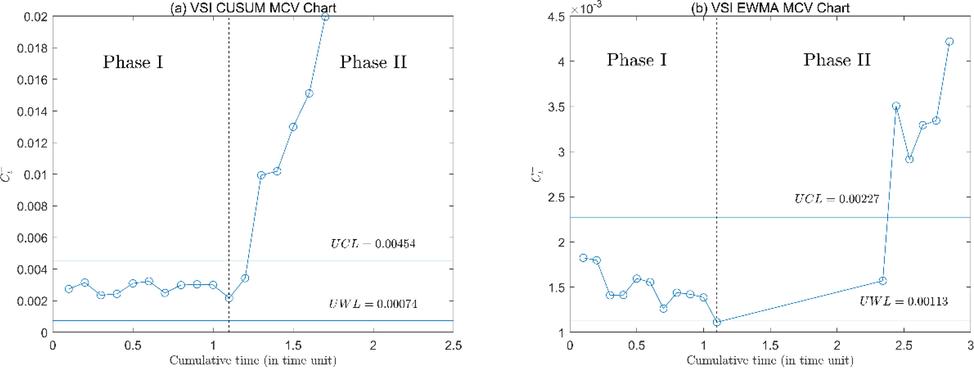
Considering the data from 2000 to 2009 as the Phase I samples, we can estimate the IC MCV as . It is the interest of the company that a shift in from to , i.e., , should be detected. Following Giner-Bosch et al. (2019), the initial values are set as and . When , , , and , the optimal parameters of the upward VSI EWMA MCV chart are computed as , and . The optimal triples of the upward VSI CUSUM MCV chart are obtained by the Eq. (25) as , and . Using Eqs. (5) and (11), the UCLs corresponding to the two charts are calculated as 0.00454 and 0.00227, respectively. The corresponding UWLs are 0.00074 and 0.00113, respectively.
The charting statistics, the sampling intervals, and the total times for the upward VSI EWMA and the upward VSI CUSUM MCV charts are presented in Table 5. Here the statistic
, the sampling interval
and the total time
correspond to the CUSUM scheme, and the statistic
,
and
correspond to the EWMA scheme. Statistics that lie in the OOC region are bolded in Table 5. Control charts based on the statistics
and
are shown in Fig. 3. As it is seen from the figure, both the EWMA and CUSUM schemes with the VSI feature make the first OOC signal at the
sample, which is the same as the upward FSI CUSUM MCV chart by Hu et al. (2023). However, the upward VSI CUSUM MCV chart, VSI EWMA MCV chart and FSI CUSUM MCV chart take 1.3 time units, 2.44 time units and 13 time units to detect the shift, respectively. The detection time taken by these charts shows that the VSI CUSUM MCV charts detect the shift faster than the FSI CUSUM MCV charts and VSI EWMA MCV charts.
0.004082
0.001824
0.1
0.1
0.002744
0.1
0.1
0.001739
0.001798
0.1
0.2
0.003146
0.1
0.2
0.000539
0.001410
0.1
0.3
0.002347
0.1
0.3
0.001422
0.001414
0.1
0.4
0.002432
0.1
0.4
0.002000
0.001594
0.1
0.5
0.003094
0.1
0.5
0.001470
0.001556
0.1
0.6
0.003227
0.1
0.6
0.000603
0.001262
0.1
0.7
0.002492
0.1
0.7
0.001834
0.001439
0.1
0.8
0.002989
0.1
0.8
0.001383
0.001421
0.1
0.9
0.003034
0.1
0.9
0.001305
0.001386
0.1
1
0.003002
0.1
1
0.000499
0.001112
0.1
1.1
0.002163
0.1
1.1
0.002599
0.001570
1.24
2.34
0.003424
0.1
1.2
0.007852
0.003506
0.1
2.44
0.009939
0.1
1.3
0.001588
0.002915
0.1
2.54
0.010189
0.1
1.4
0.004144
0.003293
0.1
2.64
0.012996
0.1
1.5
0.003456
0.003344
0.1
2.74
0.015114
0.1
1.6
0.006183
0.004218
0.1
2.84
0.019960
0.1
1.7
The upward VSI CUSUM and EWMA MCV charts applied to the dataset in Table 5.
6 Conclusions
Integrating the VSI strategy into the CUSUM scheme, this paper proposes two new one-sided charts for monitoring the MCV. Methods for performance evaluation of the proposed charts are provided in both deterministic and unknown shifts cases. Given deterministic shifts, the optimal performance of the charts is analyzed using a Markov chain approach. When the shift size is unknown, the performance of the VSI CUSUM MCV charts is evaluated using the EATS criteria with the random shifts assumed to follow a discrete uniform distribution. The performance of the charts was compared against the corresponding FSI type charts and the VSI EWMA MCV charts. A numerical comparison shows that the detection efficiency of the standard CUSUM MCV scheme is remarkably enhanced by introducing the VSI strategy and the VSI CUSUM MCV charts outperform the VSI EWMA MCV charts in most cases. Effectiveness of the proposed VSI CUSUM MCV charts is also validated through the real case application.
In the design of the proposed MCV charts, it is assumed that observations follow a multivariate normal distribution. However, this assumption may not always hold and the underlying distribution of many processes in practical applications is non-normal, see Qiu and Li (2011). Hence, future research may develop new MCV charts for the process with unknown or non-normal distributions. In addition, the application of VSI CUSUM MCV control charts when measurement errors are present is also a research direction worthy of further study.
Acknowledgements
This work was supported by National Natural Science Foundation of China (Grant number: 71802110, 72072080, 71872088, 72101123); Postgraduate Research & Practice Innovation Program of Jiangsu Province (Grant number: KYCX22_0868); The Excellent Innovation Teams of Philosophy and Social Science in Jiangsu Province (2017ZSTD022); Key Research Base of Philosophy and Social Sciences in Jiangsu Information Industry Integration Innovation and Emergency Management Research Center; NJUPT (Grant number: NY222176); Major Project of Philosophy and Social Science Research in Colleges and Universities of Jiangsu Province (Grant number: 2023SJZD019); The Humanities and Social Sciences Youth Foundation of Ministry of Education of China (Grant number: 19YJC630221); General Project of Philosophy and Social Science Research in Colleges and Universities of Jiangsu Province (Grant number: 2021SJA0299).
Declaration of Competing Interest
The authors declare that they have no known competing financial interests or personal relationships that could have appeared to influence the work reported in this paper.
References
- Efficient control charts for monitoring process CV using auxiliary information. IEEE Access.. 2020;8:46176-46192.
- [CrossRef] [Google Scholar]
- Multivariate coefficient of variation control charts in phase I of SPC. Int. J. Adv. Manuf. Technol.. 2018;99(5–8):1903-1916.
- [CrossRef] [Google Scholar]
- A novel definition of the multivariate coefficient of variation. Biometr. J. Biometrische Zeitschrift. 2010;52(5):667-675.
- [CrossRef] [Google Scholar]
- Hotelling's T2 control chart with variable sampling intervals. Int. J. Prod. Res.. 2001;39(14):3127-3140.
- [CrossRef] [Google Scholar]
- Multivariate coefficient of variation charts with measurement errors. Comput. Ind. Eng.. 2020;147:106633
- [CrossRef] [Google Scholar]
- Variable sampling interval EWMA chart for multivariate coefficient of variation. Commun. Stat. – Theory Methods. 2022;51(14):4617-4637.
- [CrossRef] [Google Scholar]
- An approach to the probability distribution of CUSUM run length. Biometrika. 1972;59(3):539-549.
- [CrossRef] [Google Scholar]
- Monitoring the coefficient of variation using EWMA charts. J. Qual. Technol.. 2011;43(3):249-265.
- [CrossRef] [Google Scholar]
- Monitoring the coefficient of variation using a variable sampling interval control chart. Qual. Reliab. Eng. Int.. 2013;29(8):1135-1149.
- [CrossRef] [Google Scholar]
- Monitoring the coefficient of variation using a variable sample size control chart. Int. J. Adv. Manuf. Technol.. 2015;80(9–12):1561-1576.
- [CrossRef] [Google Scholar]
- One-sided downward control chart for monitoring the multivariate coefficient of variation with VSSI strategy. J. Math. Fundam. Sci.. 2020;52(1):112-130.
- [CrossRef] [Google Scholar]
- A proposed variable parameter control chart for monitoring the multivariate coefficient of variation. Qual. Reliab. Eng. Int.. 2019;35(7):2442-2461.
- [CrossRef] [Google Scholar]
- An EWMA control chart for the multivariate coefficient of variation. Qual. Reliab. Eng. Int.. 2019;35(6):1515-1541.
- [CrossRef] [Google Scholar]
- New adaptive EWMA control charts for monitoring univariate and multivariate coefficient of variation. Comput. Ind. Eng.. 2019;131:28-40.
- [CrossRef] [Google Scholar]
- Monitoring multivariate coefficient of variation with individual observations. Qual. Reliab. Eng. Int.. 2022;38(8):4236-4246.
- [Google Scholar]
- Efficient CUSUM control charts for monitoring the multivariate coefficient of variation. Comput. Ind. Eng.. 2023;179:109159
- [Google Scholar]
- Monitoring the coefficient of variation: a literature review. Comput. Ind. Eng.. 2021;161
- [CrossRef] [Google Scholar]
- A control chart for the coefficient of variation. J. Qual. Technol.. 2007;39(2):151-158.
- [CrossRef] [Google Scholar]
- One-sided control charts for monitoring the multivariate coefficient of variation in short production runs. Trans. Inst. Meas. Control. 2019;41(6):1712-1728.
- [CrossRef] [Google Scholar]
- New adaptive control charts for monitoring the multivariate coefficient of variation. Comput. Ind. Eng.. 2018;126:595-610.
- [CrossRef] [Google Scholar]
- Run sum chart for monitoring multivariate coefficient of variation. Comput. Ind. Eng.. 2017;109:84-95.
- [CrossRef] [Google Scholar]
- Monitoring the coefficient of variation using a variable sample size EWMA chart. Comput. Ind. Eng.. 2018;126:378-398.
- [CrossRef] [Google Scholar]
- One-sided variable sampling interval EWMA control charts for monitoring the multivariate coefficient of variation in the presence of measurement errors. Int. J. Adv. Manuf. Technol.. 2021;115(5–6):1821-1851.
- [CrossRef] [Google Scholar]
- One-sided synthetic control charts for monitoring the multivariate coefficient of variation. J. Stat. Comput. Simul.. 2019;89(10):1841-1862.
- [CrossRef] [Google Scholar]
- Variable sampling interval Shewhart control charts for monitoring the multivariate coefficient of variation. Appl. Stoch. Model. Bus. Ind.. 2019;35(5):1253-1268.
- [CrossRef] [Google Scholar]
- Distribution-free monitoring of univariate processes. Statist. Probab. Lett.. 2011;81(12):1833-1840.
- [CrossRef] [Google Scholar]
- Monitoring the multivariate coefficient of variation in presence of autocorrelation with variable parameters control charts. Qual. Technol. Quantit. Manage.. 2023;20(2):184-210.
- [CrossRef] [Google Scholar]
- Exponentially weighted moving average control schemes with variable sampling intervals. Commun. Stat. – Simulat. Comput.. 1992;21(3):627-657.
- [CrossRef] [Google Scholar]
- Phenetics of natural populations. V. Genetic correlates of phenotypic variation in the pocket gopher (Thomomys bottae) in California. J. Hered.. 1996;87(5):341-350.
- [Google Scholar]
- A survey of recent developments in the design of adaptive control charts. J. Qual. Technol.. 1998;30(3):212-231.
- [CrossRef] [Google Scholar]
- Run-sum control charts for monitoring the coefficient of variation. Eur. J. Oper. Res.. 2017;257(1):144-158.
- [CrossRef] [Google Scholar]
- Monitoring the ratio of population means of a bivariate normal distribution using CUSUM type control charts. Stat. Pap.. 2018;59(1):387-413.
- [CrossRef] [Google Scholar]
- Monitoring the coefficient of variation using variable sampling interval CUSUM control charts. J. Stat. Comput. Simul.. 2021;91(3):501-521.
- [CrossRef] [Google Scholar]
- The efficiency of CUSUM schemes for monitoring the coefficient of variation. Appl. Stoch. Model. Bus. Ind.. 2016;32(6):870-881.
- [CrossRef] [Google Scholar]
- Unbiased Estimators and Their Applications: Volume 2: Multivariate Case. Springer; 1996.
- Optimization designs and performance comparison of two CUSUM schemes for monitoring process shifts in mean and variance. Eur. J. Oper. Res.. 2010;205(1):136-150.
- [CrossRef] [Google Scholar]
- A control chart for the multivariate coefficient of variation. Qual. Reliab. Eng. Int.. 2016;32(3):1213-1225.
- [CrossRef] [Google Scholar]
- Monitoring the coefficient of variation using a variable sampling interval EWMA chart. J. Qual. Technol.. 2017;49(4):380-401.
- [CrossRef] [Google Scholar]
- Monitoring the coefficient of variation using a variable parameters chart. Qual. Eng.. 2018;30(2):212-235.
- [CrossRef] [Google Scholar]
- Variable sample size and sampling interval (VSSI) and variable parameters (VP) run sum charts for the coefficient of variation. Qual. Technol. Quantit. Manage. 2023:1-23.
- [CrossRef] [Google Scholar]
- A new exponentially weighted moving average control chart for monitoring the coefficient of variation. Comput. Ind. Eng.. 2014;78:205-212.
- [CrossRef] [Google Scholar]
Appendix A
Supplementary material
Supplementary material to this article can be found online at https://doi.org/10.1016/j.jksus.2023.102845.
Appendix A
Supplementary material
The following are the Supplementary material to this article:


