Generalized linear modelling based monitoring methods for air quality surveillance

Tahir Mahmood

doi:10.1016/j.jksus.2024.103145

View/Download PDF

Buy Reprints

PDF

Translate this page into:

Full Length Article

04 2024

:36;

103145

doi:

10.1016/j.jksus.2024.103145

Generalized linear modelling based monitoring methods for air quality surveillance

Tahir Mahmood¹

School of Computing, Engineering and Physical Sciences, University of the West of Scotland, Paisley PA12BE, Scotland, United Kingdom

Received: 2023-12-3, Accepted: 2024-2-26,

Disclaimer:
This article was originally published by Elsevier and was migrated to Scientific Scholar after the change of Publisher.

1 ORCID: 0000-0002-8748-5949.

Abstract

Rising industrial pollution, exacerbated by climate change, underscores the need for effective environmental monitoring. Leveraging sensor advancements and Birnbaum-Saunders distribution, this study introduces a novel surveillance method for environmental data, crucial for shaping impactful industrial policies. Simulation studies demonstrate the method's performance, and a case study on nitrogen oxide levels in Italy validates its efficacy in the early detection of severe air pollution events.

Keywords

Birnbaum-Saunders Regression model

Deviance residuals

Environmental Pollution

Standardized residuals

Statistical process monitoring

Show Related Articles from PubMed

1 Introduction

Nowadays, pollutants like sulphur dioxide, nitrogen oxides, carbon monoxide, and tropospheric ozone from fossil fuel combustion worsen air quality, affecting human health. Establishing a surveillance mechanism is essential to detect sudden changes in nitrogen oxides (NOx) content, emitted mainly by coal plants and vehicles, causing respiratory issues and lungs damage. Real-time control charts aid in swiftly detecting abrupt changes in air quality, emphasizing the growing importance of environmental monitoring. Several control charts have been proposed in the literature to observe environmental characteristics. Anderson and Thompson (2004) studied distance-based multivariate control charts for environmental surveillance. Barratt et al. (2007) adapted the cumulative sum (CUSUM) control chart to monitor the changes in carbon monoxide concentrations, where data was collected from Central London. Morrison (2008) explained how control charts could be employed to inspect environmental data. Gove et al. (2013) examined water supply in Southwestern Australia using X-bar and CUSUM charts. Sancho et al. (2014) used a functional data-based Shewhart control chart with run rules to monitor the air quality of urban areas. Based on an attribute control chart for the number of harmful contamination levels, Leiva et al. (2015) developed a threshold for environmental monitoring.

Paroissin et al. (2016) designed novel control charts to monitor a French river's dissolved oxygen concentration (DOC). The use of univariate and multivariate control charts to assess the water quality of the South Morava River was described by Đorđević et al. (2016). Marchant et al. (2018) presented a robust strategy employing multivariate control charts to examine the air quality of Chile. Rodríguez-Álvarez et al. (2021) proposed control charts for paper moisture content variability. Marchant et al. (2019) proposed bivariate control charts to monitor PM pollution in Santiago, and Qiao et al. (2021) designed a data quality control method for air quality monitoring in Chinese cities.

In literature, many positive asymmetry or skewness probability models are often fitted to describe air contaminant concentrations. For example, log-normal, gamma, beta, inverse Gaussian, exponential, extreme values, log-logistic, Johnson bounded system, Weibull, and Pearson distributions. However, many environmentalists preferred the log-normal model instead of others for fitting the air contaminant concentrations due to its close relation to Gaussian distribution and its physical explanation in terms of the law of proportionate effect (LPE) (Ott, 1990). Nevertheless, to rationalize the log-normal as a life distribution, Desmond (1985) proved the inaccuracy of using Cramér's biological model linked to the LPE. Recently, the Birnbaum-Saunders (BS) distribution has been getting more attention due to its close relation to the normal distribution. Moreover, Leiva et al. (2015) proved that rather than log-normal distribution, the BS distribution is an appropriate model for modelling concentrations of pollutants due to its accuracy in using Cramér's biological model. For the mathematical derivation of Cramér's biological model with respect to BS distribution, we may refer to Leiva et al. (2015). Hence, BS distribution is considered for developing the surveillance methods in this study.

The BS distribution has two parameters and is used to fit the data having positively skewed behavior (Chang & Tang, 1994). For example, the BS distribution is used to fit material fatigue data. Leiva et al. (2015) provided the environmental application of BS distribution with mathematical reasoning. It provides a theoretical rationale for the case study reported in this work and is an excellent fit for the data. Santos-Neto et al. (2012) suggested a Reparametrized Birnbaum-Saunders (RBS) distribution, which is closely related to the normal and asymmetrical distributions such as Gamma and Log-normal distributions. Many monitoring studies are designed based on the BS distribution. For example, a bootstrap control chart for BS distribution was proposed by Lio and Park (2008). Leiva et al. (2011) proposed control charts based on BS distribution to examine lifetimes. Saulo et al. (2015) developed an X-bar chart based on BS distribution. Aslam et al. (2016) presented the attribute control charts under repetitive sampling when a product's lifetime follows a BS distribution. Marchant et al. (2018) proposed robust multivariate control charts where subgroups follow a generalized Birnbaum-Saunders distribution. Khan et al. (2018) proposed a chart based on BS distribution under accelerated hybrid censoring. Marchant et al. (2019) presented bivariate control charts designed for BS-distributed data. Bourguignon et al. (2020) presented control charts to monitor the median parameter of BS distribution.

All the above studies are designed to monitor the BS-distributed response variable. However, linearly related covariates are recorded in many practical situations with the BS-distributed response variable. For example, the temperature is also measured with the average NOx concentration, and they mostly possess a linear relationship (Jayamurugan et al., 2013). Hence, it is more practical to design control charts based on the BS regression model, which can provide the platform to monitor the BS distributed response variable by keeping the linear relation of the covariate(s).

For BS distribution, regression models are based on the requirement that the original dependent variable be changed to a logarithmic scale, which may reduce the power of the study and make interpretations more challenging. To overcome these issues, Santos-Neto et al. (2012) suggested a Reparametrized Birnbaum-Saunders (RBS) distribution, which is closely related to the normal and asymmetrical distributions such as Gamma and Log-normal distributions. The regression models frequently focus on mean response and its initial scale; therefore, employing RBS distribution, the mean can be modelled with no changes like generalized linear models, but the distribution does not belong to the exponential family. Thus, a link function connects the mean response to the linear predictor, which includes the regressors and unknown parameters. Furthermore, the RBS model may also describe data with non-constant variance. With this motivation, this study proposes Shewhart control charts based on standardized and deviance residuals of the Reparametrized Birnbaum-Saunders (RBS) regression model to monitor the positive asymmetric data. Further, a simulation study is designed to assess the proposed charts' performance in terms of run length characteristics. Finally, the proposed charts are implemented on the air quality data to highlight the importance of proposed methods in environmental monitoring.

The rest of the article is presented as follows: the background of the RBS regression model is described in Section 2. Then, the Shewhart control charts are derived in Section 3. In Section 4, the results and design of the simulation study are presented. Further, Section 5 consists of implementing the proposed charts on air quality data. Finally, Section 6 is designed to conclude the findings of this research.

2 The Reparametrized Birnbaum-Saunders (RBS) regression model

Let $Y$ be a positive random variable that follows the RBS distribution proposed by Santos-Neto et al. (2012) with parameters scale/mean $(μ; μ > 0)$ and shape/precision $(δ; δ > 0)$ . Using this parameterization, the probability density function of $Y$ is given as:

(1)

f (y; μ, δ) = \frac{e x p (δ / 2) \sqrt{δ + 1}}{4 y^{3 / 2} \sqrt{π μ}} [y + \frac{δ μ}{δ + 1}] e x p (- \frac{δ}{4} [\frac{y (δ + 1)}{δ μ} + \frac{δ μ}{y (δ + 1)}]) .

The expected value and variance of

Y

are formulated as

E (Y) = μ

and

V a r (Y) = μ^{2} (2 δ + 5) / {(δ + 1)}^{2}

, respectively. It is interesting to note that the variance of

Y

is a function of the mean. Thus, the RBS distribution, like the Gamma distribution, allows us to model heteroscedasticity. Leiva et al. (2014) developed a new approach for BS modelling by using this reparameterization. They treated

Y_{1}, Y_{2}, \dots, Y_{n}

as independently RBS distributed random variables during the estimation process and designed a GLM-type statistical model as

E (Y_{i}) = μ_{i} = g^{- 1} ({x_{i}}^{T} β)

, where

{x_{i}}^{T} β

is a linear predictor;

g^{- 1} (.)

indicates the inverse of the link function, which must be positive, completely monotone, and at least twice differentiable;

β = β_{0}, β_{1}, \dots, β_{k}

denotes the vector of unknown parameters; and

x_{i} = 1, x_{i 1}, x_{i 2}, \dots, x_{ik}

are the values of the

k

independent variables

X_{1}, X_{2}, \dots, X_{k}

. It is to be noted that

{x_{i}}^{T} β

belongs to the i-th row vector of the design matrix

X

. The parameters of the established model

E (Y_{i}) = μ_{i} = g^{- 1} ({x_{i}}^{T} β)

are estimated by the maximum likelihood (ML) method. For a vector of parameters

θ = {(β^{T}, δ)}^{T}

, the log-likelihood function is given as:

(2)

l (θ; y) = l (θ) = \sum_{i = 1}^{n} l_{i} (μ_{i}, δ),

l_{i} (μ_{i}, δ) = \frac{δ}{2} - \frac{\log (16 π)}{2} - \frac{1}{2} \log (\frac{(δ + 1) {y_{i}}^{3} μ_{i}}{{(δ y_{i} + y_{i} + δ μ_{i})}^{2}}) - \frac{y_{i} (δ + 1)}{4 μ_{i}} - \frac{δ^{2} μ_{i}}{4 (δ + 1) y_{i}} .

Assuming

δ

as known, the deviance residuals (DRs) for the RBS regression model are defined as:

(3)

{DR}_{i} = s i g n (y_{i} - {\hat{μ}}_{i}) \sqrt{2} {[\log (2) - \frac{δ}{2} + \frac{(δ + 1) y_{i}}{4 {\hat{μ}}_{i}} + \frac{δ^{2} {\hat{μ}}_{i}}{4 (δ + 1) y_{i}} + \frac{1}{2} \log (\frac{δ (δ + 1) y_{i} {\hat{μ}}_{i}}{{(δ y_{i} + y_{i} + δ {\hat{μ}}_{i})}^{2}})]}^{\frac{1}{2}},

where,

{\hat{μ}}_{i}

represents the ML estimate of

μ_{i}

and

s i g n (y_{i} - {\hat{μ}}_{i})

gives the signal of the difference

y_{i} - {\hat{μ}}_{i}

. Further, the standardized residuals (SRs) are derived from the difference

y_{i} - {\hat{μ}}_{i}

and expressed as:

(4)

{SR}_{i} = \frac{y_{i} - {\hat{μ}}_{i}}{\sqrt{V a r ({\hat{Y}}_{i})}} = \frac{y_{i} - {\hat{μ}}_{i}}{\sqrt{{\hat{μ}}_{i}^{2} (2 δ + 5) / {(δ + 1)}^{2}}},

where

δ

is fixed and

{\hat{μ}}_{i}

denotes the ML estimate of

μ_{i}

. Further, the DR and SR of the RBS regression model are used to develop proposed control charts.

3 The Shewhart control charts for asymmetric data

In this section, we first introduce the RBS data-based control chart and then provide the structure of control charts based on deviance and standardized residuals of the RBS regression model (given in Equations 3–4). Moreover, the implementation of the proposed (DR-RBS and SR-RBS) charts, along with the existing (Y-RBS) chart is presented in Fig. 1.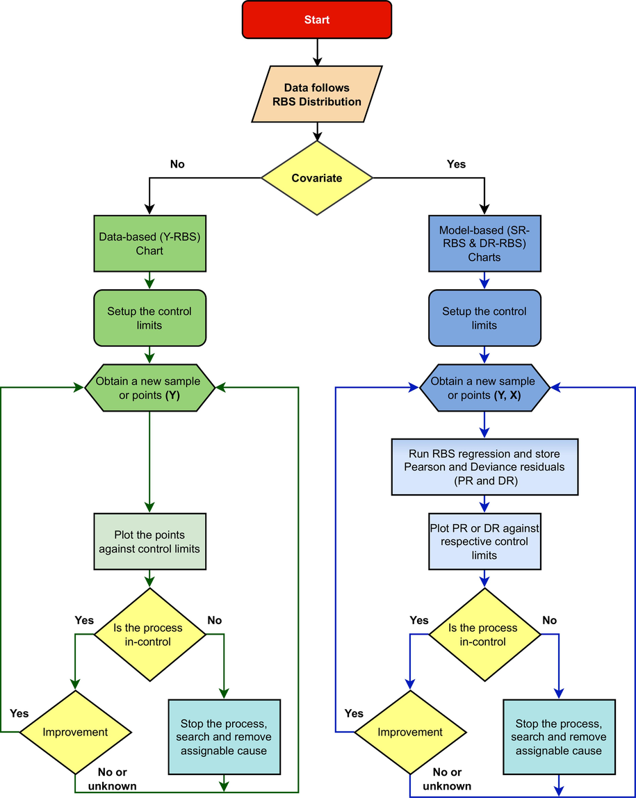

Flow chart on implementation of existing Y-RBS chart and proposed DR-RBS and SR-RBS charts.

3.1

3.1 RBS data-based control chart (Y-RBS)

The Y-RBS control chart monitors RBS distributed response variable samples, incorporating covariates, unlike the RBS data-based control chart that ignores them. The chart plots RBS samples against control limits determined by the following expression: $LCL = E (Y) - L_{Y 1} \sqrt{V a r (Y)},$

(5)

UCL = E (Y) + L_{Y 2} \sqrt{V a r (Y)},

where,

L_{Y 1}

and

L_{Y 2}

are constants that specify the width of the control limits and are set according to a fixed in-control average run length

({ARL}_{0})

. The Y-RBS chart indicates an out-of-control (OOC) state when any sample falls outside the limits; alternatively, the process reveals in-control (IC).

3.2

3.2 RBS deviance residuals based control chart (DR-RBS)

The deviance residuals of the RBS regression model are expressed in Equation (3) and plotted against the control limits in the DR-RBS control chart. The control limits of the DR-RBS chart are calculated as follows: $LCL = E (D R) - L_{D R 1} \sqrt{V a r (D R)},$

(6)

UCL = E (D R) + L_{D R 2} \sqrt{V a r (D R)},

where,

L_{D R 1}

and

L_{D R 2}

represents control limit constants and determined in relation to specified

{ARL}_{0}

. The

E (D R)

and

V a r (D R)

are the mean and variance of the deviance residuals, respectively. The DR-RBS control chart signals an OOC condition when any value of DR lies beyond the limits; otherwise, the system is considered in an IC condition.

3.3

3.3 RBS standardized residuals-based control chart (SR-RBS)

In the SR-RBS control chart, the standardized residuals stated in Equation (4) are plotted against the control limits, which are derived using the following formulas: $LCL = E (S R) - L_{S R 1} \sqrt{V a r (S R)},$

(7)

UCL = E (S R) + L_{S R 2} \sqrt{V a r (S R)},

where,

L_{S R 1}

and

L_{S R 2}

are control limit constants, and their values are selected in accordance with the defined

{ARL}_{0}

. When any value of SR exceeds the limits, the system is declared OOC; else, the system is considered IC.

Fig. 1 shows the implementation of DR-RBS, SR-RBS, and Y-RBS charts. Y-RBS is used when the dataset only contains the RBS distributed main variable. For DR-RBS and SR-RBS, fit the RBS regression model, estimate DRs and SRs using Equations (3) and (4), and calculate mean, standard deviation, and standardized residuals. Compute control limits using charting constants from Table 1 at a fixed ${ARL}_{0}$ . Plot residuals against control limits for DR-RBS and SR-RBS, and response (Y) values against Y-RBS control limits. If plotting statistics exceed boundaries, investigate for signals; otherwise, repeat for each time point data.

Table 1 Control charting constants of each chart with respect to ARL's.

Charts	Limits	${A R L}_{0}$
Charts	Limits	200	370	500
SR-RBS	$L_{S R 1}$	0.918	0.942	0.960
SR-RBS	$L_{S R 2}$	6.100	6.550	6.800
DR-RBS	$L_{D R 1}$	2.850	3.080	3.235
DR-RBS	$L_{D R 2}$	2.980	3.240	3.380
Y-RBS	$L_{Y 1}$	0.1060	0.0910	0.0843
Y-RBS	$L_{Y 2}$	11.2000	12.4000	13.3200

4 Simulation structure and results

For the performance evaluation of the proposed control charts, a Monte Carlo simulation study is designed. We generate the RBS response variable as $Y_{i} \sim R B S (μ_{i}, δ)$ , where, $μ_{i} = \exp (β_{0} + β_{1} x_{i}); i = 1, 2, \dots, n$ represents the mean function, and $δ$ is the shape parameter. By following Leiva et al. (2014), the parameters' values are considered as $β_{0} = 0.2$ , $β_{1} = 0.5$ and $δ = 2$ . Also, the sample size is set at 1000. We assume that the values of the covariate $(X)$ come from a uniform distribution with an interval $(0, 1)$ . The simulations are carried out on a large scale with $10^{4}$ repetitions. In the RBS regression model, $μ_{i}$ and $δ$ are the basic parameters, and the primary objective is to spot an increasing shift in $μ_{i}$ at a fixed $δ$ . Thus, we assess the performance of control charts by applying different direct and indirect shifts in $μ_{i}$ . The shifts are as follows:

Indirect shift in $μ_{i}$ with respect to $β_{0}$ as $β_{0} + δ$ .
Indirect shift in $μ_{i}$ with respect to $β_{1}$ as $β_{1} X + δ$ .
Direct shift in $μ_{i}$ as $μ_{i} + δ$ .

Furthermore, the capacity to detect shifts in control charts is assessed using average run length (ARL), as recommended by several prior works, e.g. (Iqbal et al., 2022a; Iqbal et al., 2022b; Mahmood, 2020; Mahmood & Erem, 2023; Mahmood et al., 2022 ). ARL represents the average number of points before an alarm. ${ARL}_{0}$ represents an in-control ARL, while ${ARL}_{1}$ indicates an out-of-control ARL. A chart is deemed superior if for a fixed ${ARL}_{0}$ , the ${ARL}_{1}$ values are minimum. The standard deviation of run length (SDRL) specifies the dispersion of a run length, whereas the MDRL reveals the median run length.

4.1

4.1 Algorithm for determining the charting constants

The following strategy is used to determine the control limit coefficients $L_{Y 1}$ , $L_{Y 2}$ , $L_{D R 1}$ , $L_{D R 2}$ , $L_{S R 1}$ , and $L_{S R 2}$ at fixed ${ARL}_{0}$ .

Begin by creating a sample of size n using the simulated RBS model, as mentioned above.
Fit the RBS regression model to the generated data and estimate the DRs and SRs shown in Equations (3) and (4).
Calculate the mean, standard deviation, and standardized residuals for the DR-RBS and SR-RBS control charts. The mean and standard error of the response variable $(Y)$ in the Y-RBS control chart.
Calculate the control limit(s) of the control chart using the estimates from step (c) and a random value as the charting constant.
Plot the residuals of DR-RBS and SR-RBS control charts against their respective control limits. Plot the Y-RBS control chart's response $(Y)$ values against the control limit.
To reach the specified ${ARL}_{0}$ , repeat steps (a-e) many times.
If the needed ${ARL}_{0}$ is not reached, return to the starting location, adjust the previous random value, and repeat steps (a-f) until it is obtained.

Using this approach, charting constants are determined for each chart against multiple ${ARL}_{0}$ options (e.g., 200, 370, and 500). Table 1 shows the obtained control charting constants.

4.2

4.2 Simulation findings

This part examined the proposed RBS model-based control chart outcomes. Tables 2-4 show the ARL, SDRL, and MDRL for various ${ARL}_{0}$ selections.

Table 2 ARL profile of the charts under an indirect shift in

μ

with respect to

β_{0}

β_{0} + δ

ARL₀	δ	DR-RBS		SR-RBS		Y-RBS
ARL₀	δ	ARL	SDRL	ARL	SDRL	ARL	SDRL
200	0	201.75	199.69	200.61	281.54	200.78	192.59
	0.1	178.54	178.54	178.63	235.61	197.04	189.76
	0.2	136.99	142.60	148.97	181.63	159.32	155.95
	0.3	96.81	100.47	111.83	129.41	117.05	114.85
	0.4	67.61	69.24	82.66	89.25	81.78	80.44
	0.5	47.82	48.56	59.70	62.39	56.90	56.09
	0.6	34.34	34.72	43.55	43.81	41.73	40.63
	0.7	25.66	25.77	31.90	31.61	30.35	29.66
	0.8	19.61	19.31	23.66	23.77	22.91	22.62
	0.9	15.07	14.76	18.55	18.52	17.55	17.19
	1	12.03	11.54	14.07	13.75	13.89	13.42
370	0	369.30	365.44	370.23	312.87	373.95	308.92
	0.1	317.81	319.49	340.63	293.76	344.57	293.22
	0.2	234.73	251.07	255.98	243.38	270.35	249.92
	0.3	167.70	180.59	176.09	177.65	187.22	183.80
	0.4	114.25	116.35	115.07	122.29	123.86	121.07
	0.5	77.76	79.51	78.46	81.36	83.83	83.20
	0.6	54.02	54.89	54.55	56.04	58.33	57.98
	0.7	38.51	39.00	39.24	40.07	42.25	41.90
	0.8	27.95	27.65	28.67	29.76	30.63	29.99
	0.9	20.95	21.03	21.78	21.77	22.81	22.14
	1	16.28	16.06	16.44	16.20	17.99	17.43
500	0	500.48	388.31	499.32	352.65	500.24	349.92
	0.1	407.95	348.96	456.61	342.12	471.45	342.46
	0.2	298.47	284.50	349.73	299.25	365.27	305.18
	0.3	202.69	207.55	241.88	233.47	257.39	240.64
	0.4	137.09	143.48	155.94	158.64	166.39	164.04
	0.5	89.37	93.64	101.61	102.90	110.83	111.02
	0.6	62.10	63.96	69.68	71.22	76.20	77.02
	0.7	43.32	44.40	48.40	49.40	52.82	52.54
	0.8	31.61	31.77	34.11	34.20	38.11	37.49
	0.9	24.12	23.63	25.67	25.39	28.60	28.25
	1	17.79	17.55	19.42	19.16	21.47	20.84

Table 3 ARL profile of the charts under an indirect shift in

μ

with respect to

β_{1}

β_{1} X + δ

ARL0	δ	DR-RBS		SR-RBS		Y-RBS
ARL0	δ	ARL	SDRL	ARL	SDRL	ARL	SDRL
200	0	201.75	199.69	200.61	281.54	202.43	195.69
	0.1	179.99	237.03	180.37	178.89	196.70	194.05
	0.2	138.40	141.77	147.00	181.04	159.15	157.87
	0.3	97.30	98.68	114.33	132.57	115.50	115.32
	0.4	67.15	68.38	83.00	89.41	81.68	79.99
	0.5	47.97	48.21	61.12	63.14	57.64	56.76
	0.6	34.15	34.42	43.45	44.43	41.56	41.30
	0.7	25.22	20.11	31.93	32.58	30.51	30.23
	0.8	19.34	19.23	23.70	23.71	22.98	22.46
	0.9	14.97	14.55	18.52	18.20	17.66	17.31
	1	11.90	11.60	14.11	13.75	14.00	13.53
370	0	369.30	365.44	370.23	312.87	376.76	309.24
	0.1	314.32	319.01	339.65	293.47	347.22	295.21
	0.2	238.98	251.99	255.12	242.62	270.98	247.94
	0.3	168.18	183.03	176.95	178.92	182.39	180.03
	0.4	113.63	119.47	115.64	120.10	121.71	120.77
	0.5	76.45	78.15	76.97	79.37	82.92	82.30
	0.6	53.33	54.31	53.64	55.40	57.89	58.49
	0.7	37.99	37.79	39.07	40.01	42.02	41.37
	0.8	27.77	27.60	28.63	28.58	30.96	30.25
	0.9	21.18	20.89	21.87	22.05	22.82	21.97
	1	16.48	16.25	16.79	16.62	18.05	17.53
500	0	500.48	388.31	499.32	352.65	505.54	350.77
	0.1	405.59	348.81	462.76	341.70	471.53	342.95
	0.2	300.50	285.10	355.15	305.08	369.35	307.13
	0.3	203.73	206.48	240.46	234.16	259.43	241.30
	0.4	139.32	145.44	155.58	156.36	168.19	168.15
	0.5	88.97	91.62	100.23	100.85	111.31	112.12
	0.6	61.45	63.39	67.54	69.07	76.77	76.36
	0.7	43.56	44.36	48.42	49.19	53.09	52.36
	0.8	31.31	31.88	34.54	34.36	39.00	38.00
	0.9	23.50	23.70	25.86	26.12	28.28	27.79
	1	18.04	17.80	19.58	19.34	21.66	21.21

Table 4 ARL profile of the charts under a direct shift in

μ

μ + δ

ARL₀	δ	DR-RBS		SR-RBS		Y-RBS
ARL₀	δ	ARL	SDRL	ARL	SDRL	ARL	SDRL
200	0	201.75	199.69	200.61	281.54	200.95	194.41
	0.1	193.95	191.56	192.06	256.15	198.44	199.77
	0.2	169.70	171.75	176.28	227.36	187.35	194.55
	0.3	149.19	150.92	155.39	194.07	179.97	178.76
	0.4	125.50	127.88	137.12	169.03	155.37	152.41
	0.5	103.46	106.14	116.70	133.05	134.07	132.30
	0.6	87.95	90.10	104.08	117.79	114.59	113.99
	0.7	74.05	75.39	87.46	96.93	97.23	96.42
	0.8	63.62	64.75	77.11	85.28	82.28	81.99
	0.9	54.86	55.82	67.58	72.12	72.03	71.85
	1	47.03	48.44	59.62	62.94	62.56	61.72
370	0	369.30	365.44	370.23	312.87	370.64	309.66
	0.1	340.58	340.69	357.25	303.85	365.03	308.48
	0.2	299.80	306.57	321.67	284.30	347.52	294.31
	0.3	256.84	270.31	273.94	254.39	311.16	274.94
	0.4	212.53	227.93	232.48	224.58	258.98	240.72
	0.5	178.13	194.30	185.80	184.71	220.74	211.06
	0.6	148.36	158.89	153.76	157.36	182.57	177.04
	0.7	126.38	134.53	127.05	131.97	152.16	150.41
	0.8	106.29	112.33	107.98	112.83	127.39	125.25
	0.9	89.47	93.42	90.26	92.08	107.52	106.56
	1	76.23	77.79	79.13	83.23	91.43	91.17
500	0	500.48	388.31	499.32	352.65	503.04	348.33
	0.1	449.19	365.70	487.33	347.91	495.20	350.32
	0.2	398.04	342.59	439.62	339.06	471.40	344.31
	0.3	324.02	301.57	382.44	315.35	416.92	325.93
	0.4	269.12	265.10	314.51	282.33	362.24	302.94
	0.5	223.75	225.08	258.55	246.45	306.45	272.57
	0.6	178.93	184.59	208.54	206.73	246.93	233.61
	0.7	147.33	154.54	172.67	174.04	207.13	199.05
	0.8	122.88	129.79	142.74	145.14	171.62	167.02
	0.9	107.03	112.30	119.10	121.38	145.48	143.81
	1	90.08	92.61	102.06	105.14	123.19	121.21

Table 2 shows the results of the first indirect shift in μ relative to $β_{0}$ as $β_{0} + δ$ across all charts. Model-based charts outperform data-based charts in detecting indirect mean shifts caused by $β_{0}$ changes. For example, when $δ = 0.7$ , the ${ARL}_{1}$ for Y-RBS chart is reported as 30.35. This is greater than the ${ARL}_{1}^{'} s$ of 25.66 and 31.90 for DR-RBS and SR-RBS charts, respectively, at fixed ${ARL}_{0} = 200$ . The shift leads ${ARL}_{1}^{'} s$ about 38.51, 39.24, and 42.25 for DR-RBS, SR-RBS, and Y-RBS control charts, respectively, at ${ARL}_{0} = 370$ . At ${ARL}_{0} = 500$ . , DR-RBS, SR-RBS, and Y-RBS charts show reductions of 456.68, 451.6, and 447.18 units, respectively. The results also reveal that in model-based charts, the deviance residuals-based scheme performs better than the standardized residuals-based scheme.

For example, at $δ = 0.2$ , the DR-RBS chart's ${ARL}_{1}$ is 136.99, whereas the SR-RBS chart's ${ARL}_{1}$ is 148.97 at ${ARL}_{0} = 200$ . For DR-RBS and SR-RBS control charts, the depreciated ${ARL}_{1}^{'} s$ are reported at roughly 234.73 and 255.98, respectively, at the given ${ARL}_{0} = 370$ . Similarly, with ${ARL}_{0} = 500$ , the shift may result in a decrease of 201.53 and 150.27 units in ${ARL}_{1}^{'} s$ of DR-RBS and SR-RBS control charts.

Table 3 summarizes the indirect change in $μ$ with respect to $β_{1}$ as $β_{1} X + δ$ across all charts. The results indicate that residuals-based procedures outperform data-based methods in detecting indirect changes in the mean induced by varying $β_{1}$ . At $δ = 0.6$ , the DR-RBS, SR-RBS, and Y-RBS charts show ${ARL}_{1}^{'} s$ around 34.15, 43.45, and 41.56, respectively, with stated ${ARL}_{0} = 200$ . While the ${ARL}_{1}^{'} s$ of DR-RBS, SR-RBS, and Y-RBS charts are seen as 53.33, 53.64, and 57.89, respectively, for ${ARL}_{0} = 370 .$ The shift may reduce the values of ${ARL}_{1}^{'} s$ for DR-RBS, SR-RBS, and Y-RBS charts by 438.55, 432.46, and 423.23 units, respectively, at ${ARL}_{0} = 500$ .

Furthermore, the results show that the deviance residuals-based process performs more effectively than the standardized residuals-based method. For example, when $δ = 0.1$ , the ${ARL}_{1}^{'} s$ are reported around 179.99 and 180.37 for DR-RBS and SR-RBS control charts, respectively, at ${ARL}_{0} = 200$ . For DR-RBS and SR-RBS control charts, ${ARL}_{1}^{'} s$ are reported around 314.32 and 339.65, respectively, with ${ARL}_{0} = 370$ . At ${ARL}_{0} = 500$ , DR-RBS and SR-RBS control charts show a drop of 94.41 and 37.24, respectively, for the same shift.

Table 4 shows the findings for direct shifts in $μ$ as $μ + δ$ . Again, techniques relying on RBS model residuals outperform the RBS data-based approach in detecting direct alterations in the mean. For example, when δ = 0.5, the DR-RBS, SR-RBS, and Y-RBS control charts constitute ${ARL}_{1}^{'} s$ around 103.46, 116.70, and 134.07, respectively, at ${ARL}_{0} = 200$ . For ${ARL}_{0} = 370$ , the ${ARL}_{1}^{'} s$ of the DR-RBS, SR-RBS, and Y-RBS control charts are 178.13, 185.80, and 220.74, respectively. The shift may have caused a drop of approximately 276.25, 241.45, and 193.55 units in the ${ARL}_{1}^{'} s$ of DR-RBS, SR-RBS, and Y-RBS control charts, respectively, at ${ARL}_{0} = 500$ . Furthermore, it can be seen that the DR-RBS control chart performs better than the SR-RBS chart. For shift δ = 0.3, the ${ARL}_{1}^{'} s$ of DR-RBS and SR-RBS control charts are found at approximately 149.19 and 155.39, respectively, at ${ARL}_{0} = 200$ . For the same shift, the DR-RBS and SR-RBS control charts exhibit ${ARL}_{1}^{'} s$ around 256.84 and 273.94, respectively, at ${ARL}_{0} = 370$ . Similarly, at ${ARL}_{0} = 500$ , the DR-RBS and SR-RBS control charts fall by 175.98 and 117.56 units, respectively. To summarize, the DR-RBS control chart outperforms the SR-RBS and Y-RBS control charts for all three types of shifts.

5 Illustrative Example: Air quality data

The simulation revealed higher detection ability in the proposed model-based (DR-RBS and SR-RBS) charts compared to the existing data-based (Y-RBS) charts, with the DR-RBS outperforming SR-RBS and Y-RBS across various shift types. To assess real-world performance, we conducted a case study using air quality data from De Vito et al. (2009), who utilized a multisensor system weighing less than 2.5 kg. This system included a relative humidity sensor, a solid-state temperature sensor, and five unique metal oxide chemo-resistive sensors, collecting data with an 8-second sampling time and a memory capacity of up to 72 h. Genuine NOx concentrations were measured on-site using a conventional analyzer as used in this study.

As previously discussed in Section 1, in order to monitor air pollution, a surveillance system must be designed to identify a sudden shift in NOx concentration while also taking temperature into account. The website (https://archive.ics.uci.edu/ml/datasets/air+quality) provides actual hourly averaged nitrogen oxides (NOx) concentration ( $Y$ , in ppb) and temperature ( $X$ , in °C). The collection contains 9358 instances of hourly averaged answers from a metal oxide chemical sensor embedded in an air quality chemical device. The device was located on a field at street level in a very polluted area of an Italian city.

For the implementation of the proposed charts, two datasets were first retrieved, each of 950 values. The dataset with an RBS distribution is considered in-control (IC), whilst the other is considered out-of-control (OOC). The descriptive statistics for nitrogen oxides (NOx) concentration in the IC dataset show that: (i) the minimum and maximum values are 2.0 and 396.0, respectively; (ii) the mean and standard deviation are 119.2095 and 79.7717, respectively; and (iii) the coefficient of variation with skewness and kurtosis are 0.6692, 1.2529, and 4.2629. These descriptive statistics show that the NOx data have a positive skew empirical distribution with a somewhat higher kurtosis than a normal (or Gaussian) distribution. The histogram in Fig. 2 illustrates these data aspects by approximating the probability density function of nitrogen oxide concentration. The QQ Plot is a popular approach for determining sample data's goodness-of-fit to a theoretical distribution. It enables the user to compare an empirical quantile function (represented by all sample points) to a theoretical model (represented by a 45° slope line). All of the data points are then compared to a straight line. If the line closely fits the point, the distribution is said to be best suited. Fig. 3 shows a QQ plot with an envelope to evaluate the model's distributional assumption.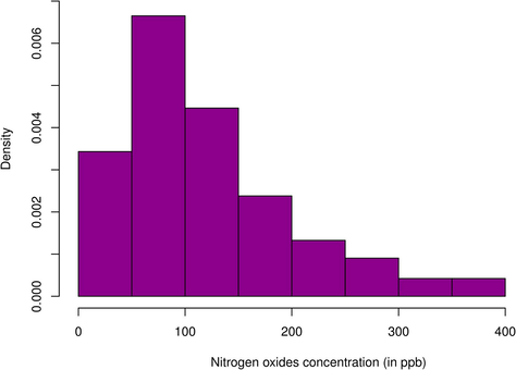

Histogram of Nitrogen Oxides (NOx) concentration.

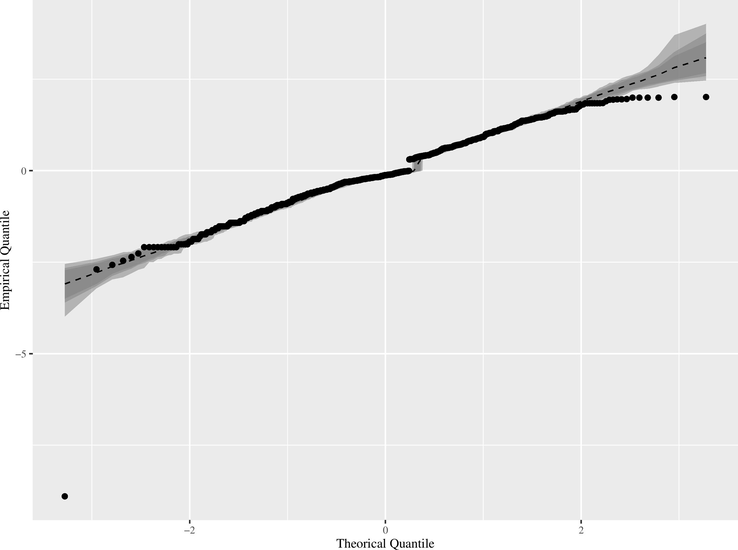
QQ plot for IC RBS regression model with Envelope.

Because this plot does not show odd features, the assumption that the response variable follows an RBS distribution is validated. Further, to analyze the model fitting, we have used Anderson-Darling and Cramer-von Mises goodness-of-fit tests (Barros et al., 2014). The RBS distribution is the best-fitted distribution, according to statistic $A = 0.4948$ with $p - v a l u e = 0.2145$ and statistic $W = 0.0571$ with $p - v a l u e = 0.4132$ .

For both IC and OOC datasets, we ran RBS regression models between NOx and temperature. These models are obtained as:

(8)

ICModel : N O x = e^{5.0511 - 0.0124 (t e m p e r a t u r e)}

(9)

OOCModel : N O x = e^{5.8164 + 0.0127 (t e m p e r a t u r e)}

The intercept and slope in Equation (8) are statistically significant (p-values < 0.001). Equation (9) shows a significant intercept (p-value < 0.001) and slope (p-value < 0.05). Further deviance and standardized residuals for both models are computed using Equations (3) and (4), respectively. Control charting constants for

{ARL}_{0} = 200

are obtained by following section 4.1 and using the IC dataset. The bootstrapping approach was applied, resulting in the following values:

L_{Y_{1}} = 1.29

L_{Y_{2}} = 12.7

L_{{SR}_{1}} = 1.329, L_{{SR}_{2}} = 3.69

L_{{DR}_{1}} = 3.0

and

L_{{DR}_{2}} = 2.20

Figs. 3-4 illustrate the implementation and presentation of the Y-RBS, SR-RBS, and DR-RBS charts. The points beneath the pink window correspond to the IC state, whilst the points under the white window indicate the OOC state. Plotting data are indicated in blue for accuracy, whereas OOC points are emphasized in red. It is noted that the Y-RBS chart (Fig. 4) discovered 104 OOC signals, whereas the SR-RBS (Fig. 5) and DR-RBS (Fig. 6) charts detected 107 and 110 OOC signals. As a consequence, this provides unambiguous proof that the simulated and illustrated example findings are identical: the DR-RBS chart has more detection power than the Y-RBS and SR-RBS charts.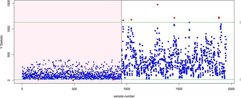

Y-RBS control chart for the illustrative example.

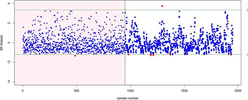
SR-RBS control chart for the illustrative example.

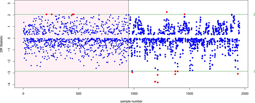
DR-RBS control chart for the illustrative example.

6 Conclusion and future recommendations

There are many real-world datasets that demonstrate positive skew behavior. For such data, symmetric distributions with support throughout the complete set of real numbers are unsuitable. To monitor positive skew data, we offer new Shewhart control charts based on the RBS regression model's residuals (SR and DR). Furthermore, a simulation study was carried out to evaluate the performance of RBS model-based control charts to the RBS data-based scheme. The findings demonstrated that RBS model-based schemes outperformed RBS data-based schemes. Furthermore, in RBS model-based schemes, the control chart, which is based on the RBS regression model's deviance residuals, is more sensitive to growing mean shifts. In conclusion, our results and application to nitrogen oxides (NOx) data offer an effective real-time monitoring tool for analyzing environmental systems. This example demonstrates the significance of the new technique in recognizing instances of severe urban environmental pollution, allowing us to avoid harmful implications for the population's health in Italy. The proposed approach is recommended for environmentalists and other administrators who wish to monitor the alarming incidence of air pollution in real-time, which is critical for human safety.

The current study lacks consideration of time series components, a key aspect that should be explored in future research. It focuses solely on nitrogen oxide (NOx) for air quality assessment, overlooking other vital contaminants like particulate matter, ozone, carbon monoxide, and sulfur oxides. Potential areas for further investigation include the impact of parameter estimation in the RBS regression model, assumptions regarding covariates in mean calculation, and the use of RBS regression modeling for skewed data detection.

Ethical approval

This article does not contain any studies with human participants or animals performed by any of the authors.

CRediT authorship contribution statement

Conceptualization, Data curation, Writing – original draft, Writing – review & editing, Visualization, Investigation, Validation, Formal analysis, Methodology.

Acknowledgement

The author is thankful to the University of the West of Scotland for providing research facilities for conducting this research.

Declaration of competing interest

The authors declare that they have no known competing financial interests or personal relationships that could have appeared to influence the work reported in this paper.

References

Anderson M.J., Thompson A.A., . Multivariate control charts for ecological and environmental monitoring. Ecol. Appl.. 2004;14(6):1921-1935.
[Google Scholar]
Aslam M., Arif O.H., Jun C.-H., . An attribute control chart based on the birnbaum-saunders distribution using repetitive sampling. IEEE Access. 2016;4:9350-9360.
[Google Scholar]
Barratt B., Atkinson R., Anderson H.R., Beevers S., Kelly F., Mudway I., Wilkinson P., . Investigation into the use of the CUSUM technique in identifying changes in mean air pollution levels following introduction of a traffic management scheme. Atmos. Environ.. 2007;41(8):1784-1791.
[Google Scholar]
Barros M., Ospina R., Tsuyuguchi A., . Goodness-of-fit tests for the birnbaum-saunders distribution with censored reliability data. IEEE Trans. Reliab.. 2014;63(2):543-554.
[Google Scholar]
Bourguignon M., Lee Ho L., Fernandes F.H., . Control charts for monitoring the median parameter of birnbaum-saunders distribution. Qual. Reliab. Eng. Int.. 2020;36(4):1333-1363.
[Google Scholar]
Chang D.S., Tang L.C., . Random number generator for the birnbaum-saunders distribution. Comput. Ind. Eng.. 1994;27(1–4):345-348.
[Google Scholar]
De Vito S., Piga M., Martinotto L., Di Francia G., . CO, NO2 and NOx urban pollution monitoring with on-field calibrated electronic nose by automatic bayesian regularization. Sens. Actuators B. 2009;143(1):182-191.
[Google Scholar]
Desmond A., . Stochastic models of failure in random environments. Canadian Journal of Statistics. 1985;13(3):171-183.
[Google Scholar]
Đorđević P., Voza D., Vuković M., . Implemetation of control charts in environmental monitoring of water quality. paper presented at the environmental awareness as a universal european value. Visegrad Project: 11540386 International Student Symposium; 2016.
Gove A.D., Sadler R., Matsuki M., Archibald R., Pearse S., Garkaklis M., . Control charts for improved decisions in environmental management: a case study of catchment water supply in south-west W estern a ustralia. Ecol. Manag. Restor.. 2013;14(2):127-134.
[Google Scholar]
Iqbal A., Mahmood T., Ali Z., Riaz M., . On enhanced GLM-based monitoring: an application to additive manufacturing process. Symmetry. 2022;14(1):122.
[Google Scholar]
Iqbal A., Mahmood T., Nazir H.Z., Chakraborty N., . On the improved generalized linear model-based monitoring methods for poisson distributed processes. Concurrency and Computation: Practice and Experience. 2022;34(11):e6889.
[Google Scholar]
Jayamurugan R., Kumaravel B., Palanivelraja S., Chockalingam M., . Influence of temperature, relative humidity and seasonal variability on ambient air quality in a coastal urban area. International Journal of Atmospheric Sciences. 2013;2013(9):1-7.
[Google Scholar]
Khan N., Srinivasa Rao G., Aslam M., . Design of chart for a birnbaum saunders distribution under accelerated hybrid censoring. J. Stat. Manag. Syst.. 2018;21(8):1419-1432.
[Google Scholar]
Leiva V., Soto G., Cabrera E., Cabrera G., . New control charts based on the birnbaum-saunders distribution and their implementation. Revista Colombiana De Estadística. 2011;34(1):147-176.
[Google Scholar]
Leiva V., Santos-Neto M., Cysneiros F.J.A., Barros M., . Birnbaum-saunders statistical modelling: a new approach. Stat. Model.. 2014;14(1):21-48.
[Google Scholar]
Leiva V., Marchant C., Ruggeri F., Saulo H., . A criterion for environmental assessment using birnbaum-saunders attribute control charts. Environmetrics. 2015;26(7):463-476.
[Google Scholar]
Lio Y.L., Park C., . A bootstrap control chart for birnbaum-saunders percentiles. Qual. Reliab. Eng. Int.. 2008;24(5):585-600.
[Google Scholar]
Mahmood T., . Generalized linear model based monitoring methods for high-yield processes. Qual. Reliab. Eng. Int.. 2020;36(5):1570-1591.
[Google Scholar]
Mahmood T., Erem A., . A bivariate exponentially weighted moving average control chart based on exceedance statistics. Comput. Ind. Eng.. 2023;175:108910
[Google Scholar]
Mahmood T., Iqbal A., Abbasi S.A., Amin M., . Efficient GLM-based control charts for poisson processes. Qual. Reliab. Eng. Int.. 2022;38(1):389-404.
[Google Scholar]
Marchant C., Leiva V., Cysneiros F.J.A., Liu S., . Robust multivariate control charts based on birnbaum-saunders distributions. J. Stat. Comput. Simul.. 2018;88(1):182-202.
[Google Scholar]
Marchant C., Leiva V., Christakos G., Cavieres M.F., . Monitoring urban environmental pollution by bivariate control charts: new methodology and case study in Santiago. Chile. Environmetrics. 2019;30(5):e2551.
[Google Scholar]
Morrison L.W., . The use of control charts to interpret environmental monitoring data. Nat. Areas J.. 2008;28(1):66-73.
[Google Scholar]
Ott W.R., . A physical explanation of the lognormality of pollutant concentrations. J. Air Waste Manag. Assoc.. 1990;40(10):1378-1383.
[Google Scholar]
Paroissin C., Penalva L., Pétrau A., Verdier G., . New control chart for monitoring and classification of environmental data. Environmetrics. 2016;27(3):182-193.
[Google Scholar]
Qiao X., Zhang Q., Wang D., Hao J., Jiang J., . Improving data reliability: a quality control practice for low-cost PM2. 5 sensor network. Sci. Total Environ.. 2021;779:146381
[Google Scholar]
Rodríguez-Álvarez J.L., López-Herrera R., Villalon-Turrubiates I.E., Molina-Arredondo R.D., Alcaraz J.L.G., Hernández-Olvera Ó.D., . Analysis and control of the paper moisture content variability by using fuzzy and traditional individual control charts. Chemom. Intel. Lab. Syst.. 2021;208:104211
[Google Scholar]
Sancho J., Martínez J., Pastor J., Taboada J., Piñeiro J., García-Nieto P.J., . New methodology to determine air quality in urban areas based on runs rules for functional data. Atmos. Environ.. 2014;83:185-192.
[Google Scholar]
Santos-Neto M., Cysneiros F.J.A., Leiva V., Ahmed S.E., . On new parameterizations of the birnbaum-saunders distribution. Pakistan J. Statist.. 2012;28(1):1-26.
[Google Scholar]
Saulo H., Leiva V., Ruggeri F., . Monitoring environmental risk by a methodology based on control charts. In: Theory and Practice of Risk Assessment. Springer; 2015. p. :177-197.
[Google Scholar]