A new extended distribution: properties, inference and applications in modeling of physical and natural phenomenon

Saman Hanif Shahbaz; Aisha Fayomi

doi:10.1016/j.jksus.2022.102334

View/Download PDF

Buy Reprints

PDF

Translate this page into:

Original article

11 2022

:34;

102334

doi:

10.1016/j.jksus.2022.102334

A new extended distribution: properties, inference and applications in modeling of physical and natural phenomenon

Saman Hanif Shahbaz, Aisha Fayomi

Department of Statistics, King Abdulaziz University, Jeddah, Saudi Arabia

Received: 2021-12-14, Accepted: 2022-9-17,

Disclaimer:
This article was originally published by Elsevier and was migrated to Scientific Scholar after the change of Publisher.

Peer review under responsibility of King Saud University.

Abstract

Objectives

This paper deals with an extension of the Ishita distribution alongside a new family of distributions based upon the proposed extension.

Methods

Some useful properties of the extended Ishita distribution are discussed. Estimation of the parameter has also been done by using different estimation. The extended Ishita distribution has been used to obtain a new family of distributions. Some members of the family have been discussed.

Results and conclusions

The extended Ishita distribution is applied on some real data sets to check the goodness of fit of the distribution. It is found that the proposed distribution is more suitable in modeling the data used as compared with the competing distributions.

Keywords

Ishita distribution

Moments

Entropy

T–X family

Maximum likelihood estimation

1 Introduction

The Lindley distribution; Lindley (Lindley, 1958); is a popular distribution that can be used to model asymmetrical behavior. Different authors have explored this distribution. Ghitany et al. (Ghitany et al., 2008) have studied the properties of the distribution in detail. The distribution has been generalized by Zakerzadeh H. and Dolati (Zakerzadeh and Dolati, 2009) and Nadarajah et al. (Nadarajah et al., 2011). Ghitany et al. (Ghitany et al., 2013) have proposed a power transformation of the distribution. Benkhelifa (Benkhelifa, 2017) has given yet another extension of the Lindley distribution. Some applications of the power Lindley distribution in quality control have been given by Shahbaz et al. (Shahbaz et al., 2018).

Shankar (Shanker, 2017) and Shanker and Shukla (Shanker and Shukla, 2017) have proposed the Rama and the Ishita distributions which extends the Lindley distribution. These distributions have also been extended by various authors. Garaibah and Al-Omari (Garaibah and Al-Omari, 2019) have used the transmutation technique of Shaw and Buckley (Shaw and Buckley, xxxx) to propose the transmuted Ishita distribution. Alhyasat et al. (Alhyasat et al., 2021) have given an extension of the Rama distribution with wider applicability.

Extensions in probability distributions have attracted various authors to propose the families of distributions. Gupta et al. (Gupta et al., 1998) have proposed the exponentiated class of distributions by exponentiation of the distribution function (cdf) of any distribution. This family of distributions has been discussed in detaile by Al-Hussaini and Ahsanullah (Al-Hussaini and Ahsanullah, 2015). Alzaatreh et al. (Alzaatreh et al., 2013) have suggested a method to develop families of distributions using two random variables and is named as the T–X family of distributions. Some notable families of distributions that arise as members of the T–X family of distributions are the gamma–G family of distributions; Alzaatreh et al. (Alzaatreh et al., 2014) and Zografos and Balakrishnan (Zografos and Balakrishnan, 2009), the Lindley–G distributions by Cakmakyapan and Ozel (Cakmakyapan and Ozel, 2017) among others. The gamma–G family of distributions provides distribution of record values; proposed by Chandler (Chandler, 1952) as a special case. Alzaatreh et al. (Alzaatreh et al., 2021) have also proposed a truncated version of the T–X family of distributions that provide distributions for modeling of truncated data.

2 Material and methods

The Ishita distribution is useful for modeling of continuous phenomenon. The probability density function (pdf) of this distribution is.

(1)

f (x) = \frac{θ^{3}}{θ^{3} + 2} (θ + x^{2}) \exp (- θ x); x, θ > 0

This distribution can be viewed as a mixture of exponential and gamma random variables with shape parameter 3. We will propose an extension of this distribution alongside a new family of distributions based upon that extension. The new family will be proposed by using the T–X family of distributions, proposed by Alzaatreh et al. (Alzaatreh et al., 2013) where the cdf of the new family of distributions is given as.

(2)

F_{T - X} (x) = \int_{a}^{W [G (x)]} r (t) d t = R [W \{G (x)\}]; x \in R

where $W [G (x)]$ is some absolutely continuous function of $G (x)$ and $r (t)$ is pdf of random variable T such that $a ⩽ T ⩽ b$ . Also $W (0) \to a$ and $W (1) \to b$ .

This paper deals with an extension of (1) and a new family of distributions using (2). This research is motivated by the fact that there have always been situations where the data needs some more flexible models for optimum modeling. The plan of the paper follows.

An extension of the Ishita distribution is proposed in Section 3. Section 4 contains useful properties of the proposed distribution. Parameter estimation of the distribution is given in Section 5. In Section 6, a new family of distributions has been proposed. The simulation and real data application of the Ishita distribution have been given in Section 7. Conclusions are given in Section 8.

3 The extended Ishita (EI) distribution

The pdf of Ishita distribution, with $θ = β^{- 1}$ , is.

(3)

f (x) = {[β (1 + 2 β^{3})]}^{- 1} (1 + β x^{2}) e^{- x / β}; x, β > 0

The cumulative distribution function (cdf) is. $F (x) = 1 - \frac{1 + β (2 β^{2} + 2 β x + x^{2})}{1 + 2 β^{3}} e^{- x / β}; x > 0$

The density (3) is mixture of gamma variate with shape parameter 3; $G (3, β)$ ; and exponential variate; $E (β^{- 1})$ ; with a mixing ratio of ${(1 + 2 β^{3})}^{- 1}$ . The extended Ishita distribution can be obtained by using mixture of $E (β^{- 1})$ and $G (α, β)$ with a mixing ratio of ${[1 + β^{α} Γ (α)]}^{- 1}$ , where $Γ (α)$ is the complete.

gamma function. The pdf of the extended Ishita (EI) distribution is, thus,

(4)

f_{EI} (x) = {[β \{1 + β^{α} Γ (α)\}]}^{- 1} (1 + β x^{α - 1}) e^{- x / β}; x, α, β > 0

The cdf of EI distribution is.

(5)

F_{EI} (x) = \frac{\{1 - \exp (- x / β)\} + β^{α} Γ (α, x / β)}{1 + β^{α} Γ (α)}

where

Γ (α, x_{0}) = \int_{0}^{x_{0}} w^{α - 1} e^{- w} d w

is the incomplete gamma function. This new distribution will be denoted by

E I (α, β)

. The reliability function is.

(6)

R (x) = 1 - \frac{\{1 - \exp (- x / β)\} + β^{α} Γ (α, x / β)}{1 + β^{α} Γ (α)} = \frac{\exp (- x / β) + β^{α} γ (α, x / β)}{1 + β^{α} Γ (α)}

where

γ (α, x_{0}) = \int_{x_{0}}^{\infty} w^{α - 1} e^{- w} d w = Γ (α) - Γ (α, x_{0})

The hazard rate function of is.

(7)

h (x) = \frac{f (x)}{R (x)} = \frac{x + β x^{α}}{β x + β^{α + 1} x e^{- x / β} γ (α, x / β)} .

The mode is obtained by solving $\partial \ln f (x) / \partial x = 0$ for x. Now. $\ln f (x) = - \ln [β \{1 + β^{α} Γ (α)\}] + \ln (1 + β x^{α - 1}) - \frac{x}{β}$

So $\frac{\partial \ln f (x)}{\partial x} = - \frac{1}{β} + \frac{(α - 1) β}{β x + x^{2 - α}}$ .

and hence the mode can be obtained by numerically solving. $- \frac{1}{β} + \frac{(α - 1) β}{β x + x^{α - 2}} = 0 \Rightarrow (α - 1) β^{2} - β (β x + x^{2 - α}) = 0$

The point of inflection is obtained by solving $\partial^{2} \ln f (x) / \partial x^{2} = 0$ . Now. $\frac{\partial^{2} \ln f (x)}{\partial x^{2}} = \frac{(α - 1) β [β + (α - 2) x^{1 - α}]}{(β x + x^{2 - α})}$

and hence the point of inflection can be obtained by solving $(α - 1) β [β + (α - 2) x^{1 - α}] = 0$ , for x.

The graphs of density and hazard rate function for different values of the parameters are given in Fig. 1. The graphs show that for large values of $α$ , the distribution has more than 1 points of inflection. Also, for large $α$ and small $β$ , the hazard rate function first decreases and then increases.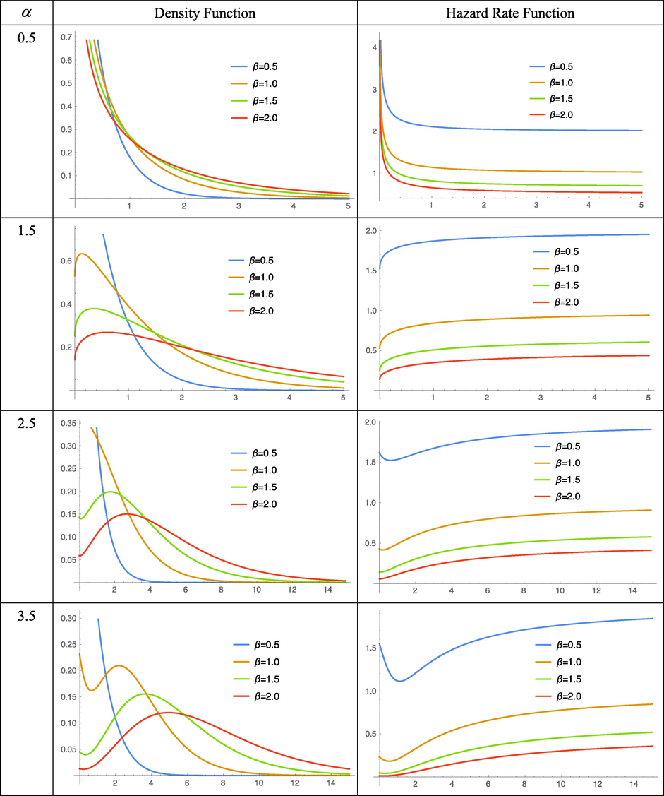

The Density and Hazard Rate Function of the Extended Ishita Distribution.

4 Distributional properties

The section deals with some properties of the EI distribution which are discussed in the following subsections.

4.1

4.1 Moments

The rth raw moment of the EI distribution is.

(8)

\begin{matrix} μ_{r}^{/} = E (X^{r}) = \frac{1}{β [1 + β^{α} Γ (α)]} \int_{0}^{\infty} x^{r} (1 + β x^{α - 1}) e x p (- \frac{x}{β}) d x \\ = \frac{β^{r} [Γ (r + 1) + β^{α} Γ (r + α)]}{1 + β^{α} Γ (α)} \cdot \end{matrix}

We can see that the above moment expression is the linear mix of the moments of exponential and gamma random variables with a mixing rate ${[1 + β^{α} Γ (α)]}^{- 1}$ . The mean and the variance of the distribution are. $μ = \frac{β [1 + β^{α} Γ (α + 1)]}{1 + β^{α} Γ (α)} and σ^{2} = \frac{β \{2 + β^{α} Γ (α + 2)\}}{1 + β^{α} Γ (α)} - {[\frac{β \{1 + β^{α} Γ (α + 1)\}}{1 + β^{α} Γ (α)}]}^{2}$

The mean and variance for the EI distribution are given in Table 1.

Table 1 Mean and Variance for EI Distribution.

Mean
$α$	$β$
$α$	0.5	1.0	1.5	2.0	2.5	3.0	3.5	4.0	4.5	5.0
0.5	0.361	0.680	0.987	1.285	1.579	1.869	2.155	2.440	2.723	3.004
1.0	0.500	1.000	1.500	2.000	2.500	3.000	3.500	4.000	4.500	5.000
1.5	0.560	1.235	1.965	2.715	3.472	4.232	4.993	5.753	6.512	7.271
2.0	0.600	1.500	2.538	3.600	4.655	5.700	6.736	7.765	8.788	9.808
2.5	0.643	1.856	3.268	4.648	5.985	7.293	8.583	9.862	11.134	12.400
3.0	0.700	2.333	4.113	5.765	7.345	8.891	10.419	11.938	13.451	14.960
3.5	0.784	2.922	4.996	6.870	8.675	10.452	12.217	13.977	15.733	17.487
4.0	0.909	3.571	5.857	7.938	9.968	11.982	13.988	15.992	17.995	19.996
4.5	1.094	4.223	6.678	8.974	11.238	13.494	15.746	17.998	20.248	22.499
5.0	1.357	4.840	7.467	9.990	12.496	14.998	17.499	19.999	22.500	25.000
Variance
$α$	$β$
$α$	0.5	1.0	1.5	2.0	2.5	3.0	3.5	4.0	4.5	5.0
0.5	0.20	0.74	1.60	2.77	4.25	6.02	8.09	10.45	13.09	16.02
1.0	0.25	1.00	2.25	4.00	6.25	9.00	12.25	16.00	20.25	25.00
1.5	0.29	1.30	3.08	5.63	8.95	13.03	17.86	23.44	29.78	36.88
2.0	0.34	1.75	4.29	7.84	12.38	17.91	24.43	31.95	40.46	49.96
2.5	0.41	2.41	5.75	10.23	15.89	22.77	30.89	40.26	50.87	62.74
3.0	0.51	3.22	7.18	12.42	19.11	27.32	37.03	48.24	60.97	75.20
3.5	0.67	4.03	8.38	14.37	22.15	31.71	43.05	56.14	70.99	87.60
4.0	0.90	4.67	9.41	16.24	25.16	36.11	49.08	64.06	81.05	100.04
4.5	1.23	5.12	10.39	18.13	28.20	40.55	55.16	72.02	91.14	112.51
5.0	1.66	5.45	11.40	20.06	31.28	45.02	61.26	80.01	101.26	125.00

From the table, we can see that, for fixed $α$ , the mean increases with an increase in $β$ . Also, for fixed $β$ , the mean increases with $α$ . The variance of the distribution exhibits the same sort of behavior. We can also see, from Table 1, that the parameter $β$ has a much larger effect on variance as compared with $α$ .

4.2

4.2 Moment generating function

The moment generating function of the distribution is. $M_{X} (t) = E (e^{tX}) = \int_{0}^{\infty} e^{tx} \frac{(1 + β x^{α - 1})}{β [1 + β^{α} Γ (α)]} \exp (- \frac{x}{β}) d x$

Using Gradshteyn and Ryzhik (Gradshteyn and Ryzhik, 2007), we have.

(9)

M_{X} (t) = \frac{{(1 - β t)}^{α} + β^{α} (1 - β t) Γ (α)}{{(1 - β t)}^{α + 1} [1 + β^{α} Γ (α)]} = \frac{{(1 - β t)}^{- 1} + β^{α} {(1 - β t)}^{- α} Γ (α)}{[1 + β^{α} Γ (α)]}

The moments can be obtained from above.

4.3

4.3 The quantile function

The quantile function is obtained by solving $F (x) = p$ for x. The quantile function for EI distribution is. $\frac{\{1 - \exp (- x / β)\} + β^{α} Γ (α, x / β)}{1 + β^{α} Γ (α)} = p$

Random sample from EI distribution can be obtained by using the quantile function.

The random sample can be obtained by direct inversion of the quantile function or by using the acceptance/rejection method with the following steps.

Use n, $α$ , $β$ and some initial value x⁰.
Obtain u from $U (0, 1)$ distribution.
Update x⁰ using $x^{*} = x^{0} - R (x^{0}; α, β)$ with $R (x^{0}; α, β) = [F_{EI} (x; α, β) - u_{0}] / f_{EI} (x; α, β)$ .
If $|x^{0} - x^{*}| < ε$ for some small $ε$ then use $x^{*}$ as a random variate from $E I (α, β)$ else set $x^{0} = x^{*}$ .
Repeat steps (2) – (4) n times to get random sample from $E I (α, β)$ .

4.4

4.4 Shannon entropy

The Shannon entropy; Shannon (Shannon, 1948); of a random variable X with density function $f (x)$ is given as $I_{S} = E [- \ln \{f (x)\}]$ . Now, for EI distribution we have. $- \ln f (x) = \ln β + \ln [1 + β^{α} Γ (α)] - \ln (1 + β x^{α - 1}) + \frac{1}{β} x$

and hence Shannon entropy for EI distribution is. $\begin{matrix} I_{S (EI)} = I_{S} (α, β) = \int_{0}^{\infty} [\ln β + \ln \{1 + β^{α} Γ (α)\} - \ln (1 + β x^{α - 1}) + \frac{1}{β} X] \\ \times \frac{1}{β [1 + β^{α} Γ (α)]} (1 + β x^{α - 1}) \exp (- \frac{x}{β}) d x . \end{matrix}$

Solving above integral, we have.

(10)

I_{S} (α, β) = \ln β + \ln \{1 + β^{α} Γ (α)\} - I + \frac{1 + β^{α} Γ (α + 1)}{1 + β^{α} Γ (α)}

Where $I = \int_{0}^{\infty} \ln (1 + β x^{α - 1}) f_{EI} (x) d x$ . Shannon entropy can be computed for different values of $(α, β)$ .

4.5

4.5 Réyni entropy

Réyni entropy; Réyni (Rényi, 1961); is defined as. $I_{R} (δ) = \frac{1}{1 - δ} \ln [I (δ)]; δ > 0; δ \neq 1$ $I (δ) = \int_{- \infty}^{\infty} f^{δ} (x) d x$

Now. $\begin{matrix} f^{δ} (x) = \frac{1}{β^{δ} {[1 + β^{α} Γ (α)]}^{δ}} {(1 + β x^{α - 1})}^{δ} \exp (- \frac{δ x}{β}) \\ = \frac{1}{β^{δ} {[1 + β^{α} Γ (α)]}^{δ}} \sum_{j = 0}^{\infty} \frac{Γ (δ + 1)}{j! Γ (δ - j + 1)} β^{j} x^{δ (α - 1)} \exp (- \frac{δ x}{β}), \end{matrix}$

So. $\begin{matrix} I (δ) = \int_{- \infty}^{\infty} \frac{1}{β^{δ} {[1 + β^{α} Γ (α)]}^{δ}} \sum_{j = 0}^{\infty} \frac{Γ (δ + 1)}{j! Γ (δ - j + 1)} β^{j} x^{δ (α - 1)} \exp (- \frac{δ x}{β}) d x \\ = \frac{1}{β^{δ} {[1 + β^{α} Γ (α)]}^{δ}} \sum_{j = 0}^{\infty} \frac{β^{α j + 1} Γ (δ + 1) Γ [j (α - 1) + 1]}{j! δ^{j (α - 1) + 1} Γ (δ - j + 1)}, \end{matrix}$

and hence,

(11)

I_{R} (δ) = \frac{1}{1 - δ} \ln [\frac{1}{β^{δ} {[1 + β^{α} Γ (α)]}^{δ}} \sum_{j = 0}^{\infty} \frac{β^{α j + 1} Γ (δ + 1) Γ [j (α - 1) + 1]}{j! δ^{j (α - 1) + 1} Γ (δ - j + 1)}]

Réyni entropy can be computed for different values of the parameters.

5 Parameter estimation and simulation

In this section, we have discussed estimation and simulation for the EI distribution. We have discussed three methods of estimation that include maximum likelihood and the method of moments. These estimation methods are discussed below.

5.1

5.1 Maximum likelihood estimation

Suppose $x_{1}, x_{2}, \dots, x_{n}$ be a random sample of size n from EI distribution. The likelihood function for a sample of size n is. $L F (α, β; x) = \frac{1}{β^{n} {[1 + β^{α} Γ (α)]}^{n}} \prod_{i = 1}^{n} (1 + β x_{i}^{α - 1}) \exp (- \frac{1}{β} \sum_{i = 1}^{n} x_{i})$

The log of likelihood function is. $ℓ (α, β; x) = - n \ln β - n \ln [1 + β^{α} Γ (α)] + \sum_{i = 1}^{n} \ln (1 + β x_{i}^{α - 1}) - \frac{1}{β} \sum_{i = 1}^{n} x_{i}$

The derivatives of log–likelihood function with respect to $α$ and $β$ are. $\frac{\partial}{\partial α} ℓ (α, β; x) = n [\sum_{i = 1}^{n} \frac{β x_{i}^{a - 1} \ln x_{i}}{1 + β x^{α - 1}} - \frac{β^{α} Γ (α) \{\ln β + ψ (a)\}}{1 + β^{α} Γ (α)}]$

and $\frac{\partial}{\partial β} ℓ (α, β; x) = \frac{1}{β^{2}} \sum_{i = 1}^{n} x_{i} + n [\sum_{i = 1}^{n} \frac{x_{i}^{a - 1}}{1 + β x^{α - 1}} - \frac{1}{β} - \frac{α β^{α - 1} Γ (α)}{1 + β^{α} Γ (α)}]$ .

The likelihood equations to estimate the model parameters are.

(12)

n [\sum_{i = 1}^{n} \frac{\hat{β} x_{i}^{\hat{α} - 1} \ln x_{i}}{1 + \hat{β} x^{\hat{α} - 1}} - \frac{{\hat{β}}^{\hat{α}} Γ (\hat{α}) \{\ln \hat{β} + ψ (\hat{a})\}}{1 + {\hat{β}}^{α} Γ (\hat{α})}] = 0

and.

(13)

\frac{1}{{\hat{β}}^{2}} \sum_{i = 1}^{n} x_{i} + n [\sum_{i = 1}^{n} \frac{x_{i}^{\hat{α} - 1}}{1 + \hat{β} x^{\hat{α} - 1}} - \frac{1}{\hat{β}} - \frac{\hat{α} {\hat{β}}^{\hat{α} - 1} Γ (\hat{α})}{1 + {\hat{β}}^{\hat{α}} Γ (\hat{α})}] = 0

The maximum likelihood estimates can be obtained by numerically solving (12) and (13). We know that the maximum likelihood estimates are asymptotically normal such that $\hat{θ} - θ$ is $N_{k} [0; I^{- 1} (\hat{θ})],$ where k is the number of parameters, $θ$ is vector of unknown parameters and $I (\hat{θ})$ is observed Fisher information matrix whose entries are given as. $I_{j, h} (θ) = - (\frac{\partial^{2}}{\partial θ_{j} \partial θ_{h}} \ln L (θ; x))$

The observed Fisher information matrix for EI distribution is. $I (α, β) = [\begin{matrix} H_{α α} & H_{α β} \\ H_{β β} \end{matrix}]$

where $H_{α α} = \partial^{2} ℓ (α, β; x) / \partial α^{2}; H_{α β} = \partial^{2} ℓ (α, β; x) / \partial α \partial β$ and $H_{β β} = \partial^{2} ℓ (α, β; x) / \partial β^{2}$ . These entries are. $\begin{matrix} H_{α α} = \frac{\partial^{2}}{\partial α^{2}} ℓ (α, β; x) = \frac{n}{{[1 + β^{α} Γ (α)]}^{2}} [β^{α} {(\ln β)}^{2} Γ (α) + 2 β^{α} (\ln β) Γ (α) ψ (α) \\ + β^{a} Γ (α) ψ^{2} (α) + β^{α} Γ (α) ψ^{/} (α) + β^{2 α} Γ^{2} (α) ψ^{/} (α) \\ - \{1 - 2 β^{α} Γ (α) - β^{2 α} Γ^{2} (α)\} \sum_{i = 1}^{n} \{\frac{β x_{i}^{α - 1} {(\ln x_{i})}^{2}}{1 + β x_{i}^{α - 1}} - \frac{β^{2} x_{i}^{2 (α - 1)} {(\ln x_{i})}^{2}}{{(1 + β x_{i}^{α - 1})}^{2}}\}] \end{matrix}$ $H_{β β} = \frac{\partial^{2}}{\partial β^{2}} ℓ (α, β; x) = n [\frac{1 + (α + 1) β^{α} Γ (α) \{2 - α + β^{α} Γ (α)\}}{β^{2} {\{1 + β^{α} Γ (α)\}}^{2}} - \sum_{i = 1}^{n} \frac{x_{i}^{2 (α - 1)}}{{(1 + β x_{i}^{α - 1})}^{2}}] - \frac{2}{β^{3}} \sum_{i = 1}^{n} x_{i}$

and. $\begin{matrix} H_{α β} = \frac{\partial^{2}}{\partial α \partial β} ℓ (α, β; x) = \frac{n}{β {[1 + β^{α} Γ (α)]}^{2}} [\sum_{i = 1}^{n} \{\frac{x_{i}^{α - 1} \ln x_{i}}{1 + β x_{i}^{α - 1}} - \frac{β x_{i}^{2 (α - 1)} \ln x_{i}}{{(1 + β x_{i}^{α - 1})}^{2}}\} \\ \times β {\{1 + β^{α} Γ (α)\}}^{2} - β^{α} Γ (α) \{1 + β^{α} Γ (α) + α \ln β + α ψ (α)\}] . \end{matrix}$

These entries can be computed for given data and hence the variance–covariance matrix of parameters $α$ and $β$ can be obtained.

5.2

5.2 Moment estimation

The EI distribution has two parameters and these can be estimated by using two moment equations $μ_{1}^{/} = m_{1}^{/}$ and $μ_{2}^{/} = m_{2}^{/}$ . Now, for EI distribution, the first two raw moments are. $μ_{1}^{/} = \frac{β [1 + β^{α} Γ (α + 1)]}{1 + β^{α} Γ (α)} and μ_{2}^{/} = \frac{β^{2} [2 + β^{α} Γ (α + 2)]}{1 + β^{α} Γ (α)}$

Equating the above raw moments with the corresponding sample moments, the moment equations are.

(14)

\frac{\hat{β} [1 + {\hat{β}}^{\hat{α}} Γ (\hat{α} + 1)]}{1 + {\hat{β}}^{\hat{α}} Γ (\hat{α})} = m_{1}^{/}

and.

(15)

\frac{{\hat{β}}^{2} [2 + {\hat{β}}^{\hat{α}} Γ (\hat{α} + 2)]}{1 + {\hat{β}}^{\hat{α}} Γ (\hat{α})} = m_{2}^{/}

The moment estimate of $β$ , when $α$ is known, can be explicitly obtained from (14) and (15). For this, we first divide (15) by square of (14) to get. $\frac{\{1 + {\hat{β}}^{α} Γ (α)\} \{2 + {\hat{β}}^{α} Γ (α + 2)\}}{{\{1 + {\hat{β}}^{α} Γ (α + 1)\}}^{2}} = \frac{m_{2}^{/}}{m_{1}^{/ 2}}$

Solving the above equation we have.

(16)

\hat{β} = {[\frac{(2 + α + α^{2} - 2 m_{2}^{/} / m_{1}^{/ 2}) \pm \sqrt{{(α - 1)}^{2} Γ^{2} (α) \{{(α + 2)}^{2} - 4 α m_{2}^{/} / m_{1}^{/ 2}\}}}{2 m_{2}^{/} Γ^{2} (α + 1) / m_{1}^{/ 2} - 2 Γ (α) Γ (α + 2)}]}^{1 / α}

which exist for ${(α + 2)}^{2} > 4 α m_{2}^{/} / m_{1}^{/ 2}$ . Also the choice between “+” or “-“ depends upon the fact that the fraction remains positive.

5.3

5.3 Simulation

This section deals with simulation study to check consistency of the estimation procedure. The simulation is conducted by generating random samples of different sizes from the EI distribution using specified values of the parameters. Estimates of $α$ and $β$ are obtained are computed using samples of different sizes and the procedure is repeated 20,000 times. The average and mean square error of the estimates are then computed to see the performance. The results are given in Table 2.

Table 2 Simulation Results for Extended Ishita Distribution.

Sample Size	True Values		Average Estimate		Mean Square Error
Sample Size	$α$	$β$	$\hat{α}$	$\hat{β}$	$\hat{α}$	$\hat{β}$
50	0.50	1.50	0.4964	1.5051	0.0836	0.2530
	2.00	3.00	1.9972	2.9976	0.3521	0.5396
	2.50	4.00	2.5025	3.9984	0.4363	0.6897
	3.50	5.50	3.4979	5.5007	0.6318	0.9717
100	0.50	1.50	0.5098	1.5066	0.0431	0.1285
	2.00	3.00	1.9989	2.9979	0.1715	0.2683
	2.50	4.00	2.4992	3.9988	0.2106	0.3387
	3.50	5.50	3.4976	5.4992	0.3076	0.4657
200	0.50	1.50	0.5048	1.5030	0.0222	0.0674
	2.00	3.00	2.0042	2.9969	0.0857	0.1264
	2.50	4.00	2.5017	3.9978	0.1073	0.1755
	3.50	5.50	3.5016	5.5018	0.1559	0.2332
500	0.50	1.50	0.5026	1.4977	0.0088	0.0261
	2.00	3.00	2.0019	3.0022	0.0353	0.0514
	2.50	4.00	2.4996	3.9992	0.0422	0.0710
	3.50	5.50	3.4978	5.5001	0.0611	0.0984
1000	0.50	1.50	0.4967	1.5019	0.0044	0.0126
	2.00	3.00	2.0035	2.9999	0.0170	0.0269
	2.50	4.00	2.5001	3.9996	0.0225	0.0358
	3.50	5.50	3.4995	5.4995	0.0294	0.0466

From above, it can be seen that the estimation is consistent.

6 A new family of distributions

This section deals with a new family of distributions by using EI distribution. The new family is proposed by using EI distribution as a distribution of T in (2). The cdf of the new family is. $F_{EI - X} (x) = \int_{0}^{W [G (x)]} \frac{(1 + β x^{α - 1})}{β [1 + β^{α} Γ (α)]} \exp (- \frac{x}{β}) d t$

or.

(17)

F_{EI - X} (x) = \frac{1}{1 + β^{α} Γ (α)} [\{1 - \exp [W \{G (x)\} / β]\} + β^{α} Γ \{α, W [G (x)] / β\}]

The pdf corresponding to (17) is.

(18)

f_{EI - X} (x) = \frac{g (x) W^{/} [G (x)] [1 + β {\{W [G (x)]\}}^{α - 1}]}{β [1 + β^{α} Γ (α)]} \exp [- \frac{1}{β} W \{G (x)\}]; x \in R

The family of distribution given above will be named as the extended Ishita–G (EI–G) family of distributions. We can see that the EI–G family of distribution is a weighted sum of exponential–G and gamma–G families of distributions.

The family of distributions given in (17) can be studied for different $W [G (x)]$ and any baseline distribution $G (x)$ . One $W [G (x)]$ that is of particular interest is. $W [G (x)] = R_{X} (x) = - \ln [1 - G (x)]$

and in this case the density function of EI – X reduces to.

(19)

f_{EI - X} (x) = \frac{g (x)}{β [1 + β^{α} Γ (α)]} [1 + β {\{R_{X} (x)\}}^{α - 1}] {[1 - G (x)]}^{1 / β - 1}; x \in R

which is a linear mix of exponentiated–G family of distributions based upon survival function and $(1 / β)$ th upper record value for $(1 / β)$ to be an integer.

7 Real data applications

In this section, we have given some data applications of the EI distribution. We have used three data sets to compare the proposed EI distribution with some existing distributions. The data sets used are Flood data based upon W; used by Akinsete et al. (Akinsete et al., 2008); the rainfall data based upon annual maximum precipitation in Korea; used by Jeong et al. (Jeong et al., 2014); and the pressure data based upon the life of fatigue fractures; used by Abdul–Moniem and Seham (Abdul-Moniem and Seham, 2015). The summary measures of three data sets are given in Table 3. We can see, from Table 3, that the data sets are positively skewed.

Table 3 Summary Measures for Various Data Sets.

Data Sets	Summary Measures
Data Sets	n	*Min*	Q₁	*Median*	*Mean*	Q₃	*Max*
Flood Data (Data 1)	72	0.100	2.125	9.500	12.204	20.125	64.000
Rainfall Data (Data 2)	105	20.7	101.6	131.6	144.6	165.5	354.7
Pressure Data (Data 3)	59	4.10	8.45	10.60	13.49	16.85	39.20

We have compared the proposed EI distribution with some existing distributions for fitting the above data sets. The distributions that we have compared are Lindley (LiD) distribution, Ishita distribution (IsD), transmuted Ishita distribution (TID), Rama distribution (RaD), exponentiated exponential distribution (EED), gamma distribution (GD) and Weibull distribution (WD); Weibull (Weibull, 1951).

We have fitted the above mentioned distributions on three data sets. The maximum likelihood estimates of parameters alongside; standard errors of estimates and some measures to see the goodness of fit for various distributions for three data sets are given in Table 4, Table 5 and Table 6. These tables also contain the values of the Akaike information criterion (AIC) and Bayesian information criterion (BIC).

Table 4 Parameter Estimates of Different Distributions for Data 1.

	α	β	SE(α)	SE(β)	LogLik	AIC	BIC
EID	0.8282	14.4735	0.1093	1.8856	−250.35	504.70	504.41
TID	0.2565	0.2382	0.1679	0.0187	−299.72	603.44	603.15
EED	0.8284	0.1024	0.1231	0.0117	−251.29	506.58	506.29
WD	0.9012	16.6323	0.0856	1.6136	−251.49	506.98	506.69
GD	0.8383	0.0987	0.1211	0.0133	−251.34	506.68	506.39
LiD	–	0.9912	–	0.5242	−2101.2	632.40	632.26
ExD	–	0.0819	–	0.0097	−252.13	506.26	506.12
IsD	–	3.9919	–	0.2696	−300.89	603.78	603.64
RaD	–	3.0643	–	0.1798	−324.93	651.86	651.72

Table 5 Parameter Estimates of Different Distributions for Data 2.

	α	β	SE(α)	SE(β)	LogLik	AIC	BIC
EID	4.7702	30.3128	0.2635	1.1076	−574.50	1153.00	1153.04
TID	−0.5748	0.0264	0.1197	0.0014	−580.89	1165.78	1165.82
EED	6.2703	0.0191	1.1059	0.0015	−582.39	1168.78	1168.82
WD	2.3186	163.408	0.1594	2.9829	−583.75	1171.50	1171.54
GD	4.7721	0.0360	0.6559	0.0047	−581.50	1167.00	1167.04
LiD	–	0.0043	–	0.2341	−621.25	1244.50	1244.52
ExD	–	0.0069	–	0.0007	−627.27	1256.54	1256.56
IsD	–	9.1196	–	0.9379	−1439.1	2880.20	2880.22
RaD	–	8.3775	–	1.4830	−1820.6	3643.20	3643.22

Table 6 Parameter Estimates of Different Distributions for Data 3.

	α	β	SE(α)	SE(β)	LogLik	AIC	BIC
EID	3.6177	3.6144	0.6634	0.7033	−188.15	380.30	379.84
TID	0.6629	0.2174	0.3114	0.0238	−193.02	390.04	389.58
EED	5.5304	0.1787	1.4292	0.0232	−191.22	386.44	385.98
WD	1.8404	15.3060	0.1713	1.1724	−197.29	398.58	398.12
GD	3.6782	0.2727	0.6530	0.0518	−193.08	390.16	389.70
LiD	–	0.4742	–	0.5812	−212.30	426.60	426.37
ExD	–	0.0741	–	0.0097	−212.51	427.02	426.79
IsD	–	2.5166	–	0.3369	−193.88	389.76	389.53
RaD	–	3.3829	–	0.2198	−193.56	389.12	388.89

The goodness of fit is also tested using Kolmogorov–Smirnov (KS) and Anderson–Darling (AD) tests. The value of test statistics alongside the p–values for various distributions are given in Table 7.

Table 7 Goodness of Fit Tests for Different Distributions.

Data	Test	Distribution
Data	Test	EID	TID	EED	WD	GD	LiD	ExD	IsD	RaD
1	KS	0.103	0.306	0.185	0.165	0.191	0.514	0.142	0.989	0.982
	*p–value*	0.428	<0.001	0.015	0.165	0.011	<0.001	0.108	<0.001	<0.001
	AD	0.766	21.884	4.355	3.270	4.691	120.309	1.459	698.64	639.10
	*p–value*	0.506	<0.001	0.006	0.020	0.008	<0.001	0.006	<0.001	<0.001
2	KS	0.093	0.135	0.172	0.126	0.136	0.642	0.301	0.903	0.886
	*p–value*	0.326	0.043	0.004	0.126	0.042	<0.001	<0.001	<0.001	<0.001
	AD	0.841	2.703	4.039	1.585	2.585	95.839	15.715	698.645	639.103
	*p–value*	0.452	0.039	0.008	0.157	0.008	<0.001	0.008	<0.001	<0.001
3	KS	0.109	0.181	0.156	0.143	0.134	0.773	0.303	0.385	0.675
	*p–value*	0.490	0.042	0.113	0.143	0.243	<0.001	<0.001	<0.001	<0.001
	AD	1.067	4.315	4.035	1.840	1.231	126.701	6.916	26.544	117.067
	*p–value*	0.324	0.006	0.008	0.113	0.008	<0.001	0.008	<0.001	<0.001

We can see from the tables that the EI distribution is most suitable for modeling the given three data sets as it has the smallest value of AIC and BIC for all three data sets as compared with the other competing distributions. We can also see that the proposed EI distribution is most suitable as it has the highest p–value for Kolmogorov–Smirnov and Anderson–Darling tests as compared with the other distributions. The histograms and empirical cdf for three data sets alongside some selected fitted distributions are given in Fig. 2. From these plots, we can see that the proposed EI distribution is the most adequate fit for the data.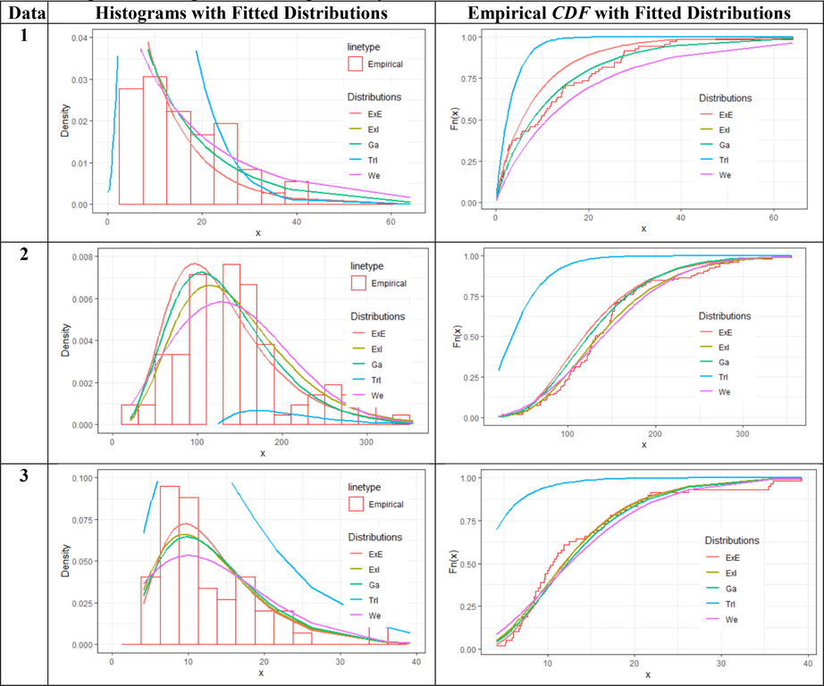

Histograms and Empirical cdf’s of Three Data Sets with Fitted Distributions.

8 Conclusions

This paper deals with a new probability distribution which extends the Ishita distribution. Ishita, Lindley and Rama distribution appear as special cases of the proposed distribution. The distribution has been studied in detail and some useful properties are discussed. Parameter estimation of the distribution is done alongside some applications. It is found that the proposed distribution fits the given data reasonably well as compared with the other distributions used in the study. A new family of distributions is also suggested by using the proposed distribution and we have found that the proposed family of distributions is a mixture of exponentiated exponential and gamma families of distributions.

Funding

This research receives no funding.

Declaration of Competing Interest

The authors declare that they have no known competing financial interests or personal relationships that could have appeared to influence the work reported in this paper.

References

Abdul-Moniem I.B., Seham M., . Transmuted Gompertz Distribution. Comp. App. Math. J.. 2015;1:88-96.
[Google Scholar]
Akinsete A., Famoye F., Lee C., . The beta-Pareto distribution. Statistics. 2008;6:547-563.
[Google Scholar]
Al-Hussaini E.K., Ahsanullah M., . Exponentiated Distributions. Paris: Atlantis Press; 2015.
Alhyasat K.M., Ibrahim K., Al-Omari A.I., AbuBakar M.A., . Extended Rama distribution: properties and applications. Comp. Sys. Sci. Engin.. 2021;39(1):55-67.
[Google Scholar]
Alzaatreh A., Lee C., Famoye F., . A new method of generating families of continuous distributions. Metron. 2013;71:63-79.
[Google Scholar]
Alzaatreh A., Famoye F., Lee C., . The gamma-normal distribution: properties and applications. Comp. Stat. Data. Ana.. 2014;69:67-80.
[Google Scholar]
Alzaatreh A., Aljarrah M.A., Smithson M., Shahbaz S.H., Shahbaz M.Q., Famoye F., Lee C., . Truncated family of distributions with applications to time and cost to start a business. Method. Comput. In App. Prob.. 2021;23:5-27.
[Google Scholar]
Benkhelifa L., . The Marshall-Olkin extended generalized Lindley distribution: Properties and applications. Comm. Stat. Sim. Comput.. 2017;46(10):8306-8330.
[Google Scholar]
Cakmakyapan S., Ozel G., . The Lindley family of distributions: properties and applications. Hacettepe J. Math. Stat.. 2017;46:1-27.
[Google Scholar]
Chandler K.N., . The distribution and frequency of record values. J. Royal Statist. Soc. B. 1952;14:220-228.
[Google Scholar]
Garaibah M., Al-Omari A.I., . Transmuted Ishita distribution and its applications. J. Stat. App. Prob.. 2019;8(2):67-81.
[Google Scholar]
Ghitany M.E., Atieh B., Nadarajah S., . Lindley distribution and its application. Math and Comp. in Sim.. 2008;78(4):493-506.
[Google Scholar]
Ghitany M.E., Al-Mutairi D.K., Balakrishnan N., Al-Enezi L.J., . Power Lindley distribution and associated inference. Comp. Stat. & Data Analysis. 2013;64:20-33.
[Google Scholar]
Gradshteyn S., Ryzhik I.M., . Table of Integrals, Series, and Products. New York.: John Wiley; 2007.
Gupta R.C., Gupta P.L., Gupta R.D., . Modeling failure time data by Lehman alternatives. Comm. Stat. Theory. Methods.. 1998;27:887-904.
[Google Scholar]
Jeong B.Y., Seo Y.A., Murshed M.S., Park J.S., . A three-parameter kappa distribution with hydrologic application: a generalized Gumbel distribution. Stoch. Environ. Res. Risk Assess.. 2014;28:2063-2074.
[Google Scholar]
Lindley D.V., . Fiducial distributions and Bayes theorem. J. Royal Stat Soc.. 1958;20(1):102-107.
[Google Scholar]
Nadarajah S., Bakouch H.S., Tahmasbi R., . A generalized Lindley distribution. Sankhya B. 2011;73:331-359.
[Google Scholar]
Rényi, A. On measures of entropy and information, in: Proceedings of the Fourth Berkeley Symposium on Mathematical Statistics and Probability, 1961, The Regents of the University of California.
Shahbaz S.H., Khan K., Shahbaz M.Q., . Acceptance sampling plans for finite and infinite lot size under power Lindley distribution. Symmetry. 2018;10 paper 496
[Google Scholar]
Shanker R., . Rama distribution and its applications. Int. J. Stat and App.. 2017;7(1):26-35.
[Google Scholar]
Shanker R., Shukla K.K., . Ishita distribution and its application. Biomet. Biostatist. Int. J.. 2017;5(2):39-46.
[Google Scholar]
Shannon C.E., . A Mathematical Theory of Communication. Bell Sys. Tech. J.. 1948;27:379-423.
[Google Scholar]
Shaw, W.T. and Buckley, I.R.C. The alchemy of probability distributions: beyond Gram-Charlier expansions, and a skew-kurtotic-normal distribution from a rank transmutation map, Research report.
Weibull W., . A Statistical Distribution Function of Wide Applicability. J. of App. Mech.. 1951;18:293-297.
[Google Scholar]
Zakerzadeh H., Dolati A., . Generalized Lindley distribution. J. Math. Extension.. 2009;3:13-25.
[Google Scholar]
Zografos K., Balakrishnan N., . On families of beta- and generalized gamma-generated distributions and associated inference. Stat. Method.. 2009;6:344-362.
[Google Scholar]