

Translate this page into:
The impact of transformations on the performance of variance estimators of finite population under adaptive cluster sampling with application to ecological data
⁎Corresponding author. hameedali@aup.edu.pk (Hameed Ali)
-
Received: ,
Accepted: ,
This article was originally published by Elsevier and was migrated to Scientific Scholar after the change of Publisher.
Abstract
This paper aims to investigate the impact of transformed auxiliary variables on the performance of variance estimators of finite population under adaptive cluster sampling scheme. Further, the formulation of an efficient variance estimator of a finite population is also under consideration in this article. Specifically, we explore the gain in efficiency obtained through various transformations and define dominance space for each transformation. These dominance regions provide valuable insights into the circumstances under which one transformation prevails over another regarding precision and accuracy. The theoretical properties of the suggested estimators have been discussed along with the dominance region under each transformation. The bias and Mean Square Error (MSE) have been derived up to the first order of approximation. To evaluate and empirically validate our methodology, we conduct a numerical analysis using real-life ecological data of blue-winged teal. The finding reflects the superior performance of the suggested variance estimators over the competing estimators, thereby substantiating its importance in making informed decisions in real-world applications.
Keywords
Adaptive cluster sampling
Auxiliary information
Transformation
Dominance region
MSE
Simulation study

1 Introduction
Sampling plays a vital role in making informed decisions in real-life domains. Inferences about the statistical population or data are based on the information extracted from the sample. Therefore, a sample must be representative, mirroring every characteristic of the population of interest (Lohr, 2021). Consequently, special care must be taken in selecting a representative sample at the design and estimation stage. Adaptive cluster sampling (ACS) is of prime importance in the field of survey sampling, in situations when the variable of interest is rare, clumpy, and clustered with localized variability (Smith et al., 1995). Unlike traditional sampling methods like simple, systematic, and stratified random sampling, select units in the sample without observing it, resulting in high bias and mean square error. ACS allows the dynamic adjustment of sampling effort based on observed values to satisfy some pre-determined condition C(yi >0), thereby enhancing the efficiency of data collection as well as parameter estimation in specific contexts. This paper investigates the domain of ACS, with a specific emphasis on the use of transformed auxiliary variables to formulate efficient variance and enhance efficiency Fig. 1.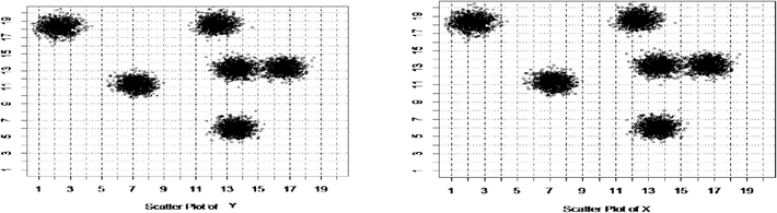
Plot of survey variable (y) and auxiliary variable (x) in study region partitioned in 20*20 square cells generated by population-1.
In survey sampling, practitioners and researchers face the challenge of optimizing sampling efforts to gather meaningful data and estimate parameters precisely. The problem becomes more challenging in a situation when the population is rare and clustered where conventional sampling efforts like simple random sampling, systematic random sampling, etc. lose their effectiveness and result in high bias and low efficiency in estimating parameters (Thompson, 1990). Therefore, the use of conventional sampling strategies leads us to doubtful and misleading inferences. This inadequacy of the design and estimation problem of classical sampling methods demands the exploration of innovative methods at both the design and estimation stages. Such as ACS and the adequate use of auxiliary information in combination with the main study variable can cater to dynamic sampling requirements. It is revealed from the numerical analysis that the precision and efficacy of estimates of the variance of finite population under ACS can be enhanced remarkably.
The main objective of this study is to assess the impact of transformed auxiliary variables on the performance of variance estimators within the framework of ACS with implications for various persuasions, such as ecology, epidemiology, and geology, where ACS can offer enhanced insights into clustered or rare populations (Thompson, 1990). In this context, several sampling survey statisticians have done their remarkable contributions. (Diggle et al., 1976) works is regarded as a pioneered distance-based approach to assess spatial event randomness using adaptive cluster sampling. The work done by (Thompson, 1990) brings further innovation to sampling designs and unbiased estimators. In estimating parameters (Chao, 2004; Félix-Medina and Thompson, 2004) explored the importance of incorporating auxiliary variables in enhancing the efficiency of ratio estimators of population mean. The work done by (Chutiman et al., 2013),(Grover and Kaur, 2014), and later by (Yadav et al., 2016) encouraged the use of transformed auxiliary variables in the efficient formulation of estimators of parameters. A similar strategy of incorporating a transformed auxiliary variable with the study variable can also be seen in the work of (Gattone et al., 2016) for rare and clustered populations. (Noor-Ul-Amin et al., 2018) and (Yasmeen et al., 2018) suggested an effective variance estimator under adaptive cluster sampling (ACS) and Stratified adaptive cluster (SACS) sampling. Some recent work in the field of survey sampling on efficient formulation of variance under adaptive cluster sampling is due (Qureshi et al., 2020; Singh & Mishra, 2022; Yasmeen et al., 2022), (Ahmad et al., 2021), (Qureshi et al., 2020), (Singh and Mishra, 2022) with diverse applications specifically to ecological data and health data including COVID-19.
2 Methodology
Let us consider the population P of size N, where . Let an initial sample of size n be drawn from the population using a Simple random sampling without replacement (SRSWOR) scheme such that . Let , be the unit observed in the initial sample of the main study variable and supplementary variable . The supplementary variable where is supposed to be positively correlated with the study variable , where .
The selection of units in the primary sample and its neighboring components is based on some predefined condition , according to ACS. If the unit selected by SRSWOR and observed satisfies the condition it is included in the sample. The additional sampling units vary adaptively selected in this way. A network of sampling units is therefore selected, consisting of all components that satisfy those conditions. The neighbouring components that fail to satisfy the condition , is called the edge component. The network with its edge component is called a cluster, as a whole. The networks formed so, are non-overlapping and comprise the whole population.
Consider a network
consisting of
components. Let
be the
network in the population contains component j. let us denote the average values of the elements of variables y and x by
and
respectively, as following
Suppose,
,
error due to sampling of main study variable y and supplementary variable x respectively.
is a finite population correction factor (fpc).
and
are the sample mean of
and
respectively.
is the second-order moments and (r, q) is the non-negative integers.
and
are the coefficients of kurtosis due to y and x respectively.
is the moment ratio?
,
The average of auxiliary variable x belonging to the sample
where
and
is the collection of all samples.
and
be the average values of the elements in the kth-network for variable
and x, respectively.
and
respectively.
and
be the sample variances and
and
be the population variances of y and x respectively.
-
The usual variance estimator of population variance is given by
Which is an unbiased estimator with variance given by
By letting .
-
(Isaki, 1983) suggested the ratio estimator of population variance in ACS design as follows
-
(Yasmeen and Thompson, 2020) proposed the following class of estimators of finite population variance as following
Where are some suitable constants or some functions of auxiliary variables?
The Bias and MSE of
is given by
(7)
Where
for different choices of
,
takes the following special form listed in Table 1.
S.No
Estimator
Bias and MSE
1
2
3
4
5
3 Proposed estimators
Motivated by (Isaki, 1983), the first estimators is proposed by taking the linear combination of usual ratio and exponential estimators in term of transformed auxiliary variable, and similarly in the second estimator is proposed by taking the linear combination of regression ratio and exponential form of transformed auxiliary variable with the main study variable as following
Transformed Auxiliary Variable
Error term
Transformer/normalizers
Properties of Error term
Dominance region
and both
4 Asymptotic properties of the proposed estimators
The theoretical properties of the developed estimators are discussed along with the transformations given in Table 1, the properties of the error term will alter with each transformation and accordingly influence the sampling error as given in Table 3. Their corresponding superiority or dominance space bounds the validity of the transformation properties of the error due to sampling using the transformed auxiliary variable, we can now obtain the bias and mean square error (MSE) of
and
,k=1,2,..,7., Rewriting eq.(9) and eq. (10) in terms of the error due to sampling as following Table 4.
0
0
3
5
0
0
0
0
0
0
0
0
0
24
14
0
0
10
103
0
0
0
0
0
2
3
2
0
13,639
1
0
0
0
0
0
0
0
37
14
122
0
0
0
0
0
0
2
0
0
177
0
0
11
17
0
0
0
0
0
0
0
0
0
95
51
0
0
39
422
0
0
0
0
0
9
12
7
0
54,483
4
0
0
0
0
0
0
0
0
53
499
0
0
0
0
0
0
9
0
0
734
5 Theoretical comparisons
The theoretical comparison of the first and second proposed class of estimators given by eq.(9) to eq.(10) for k=1,2,…,6. against the competing estimators given by eq.(2), eq.(5) and eq.(8) and some special cases of eq.(8) for i=1,2,…,5., discussed in the literature under adaptive cluster sampling is given as following:
-
The proposed estimator given by eq.(9) and eq.(10) well outperform the usual classical estimator given by eq.(2) in ACS, if
and
Or .
and
-
The proposed estimator given by eq.(9) and eq.(10) will outperform the ratio type estimator given by eq.(5) if
And
Or
And
-
The proposed estimator will outperform the ratio type transformed class of estimator given by (8) and with special cases given in Table1 if
The above conditions hold true for all types of data when there is a positive correlation between the main survey variable and auxiliary variable.
6 Numerical analysis
The performance of the proposed estimator against competing estimators was demonstrated in a simulation study under the ACS design. Two populations were used: a Poisson cluster (Diggle et al., 1976) pages 55–57. Second population is taken from (Smith et al., 1995) in which 5000 km2 of area distributed among quadrants in central Florida. The data of blue-winged teal was used as an auxiliary variable to compare the efficiency of the estimators and the estimator suggested by (Isaki, 1983) in estimating variance under adaptive cluster sampling without replacement sampling. Denoting the j-th variate of interest and auxiliary variate by and . (Dryver & Chao, 2007).
The following two models generated the survey variable, given by
The following steps are used in R-Language to perform simulation:
Step 1: Generate response variable y using model (21) and (22) with supplementary variable x and from given populations.
Step 2: Consider initial sample sizes for 100,000 repetitions to calculate the variance estimator in adaptive cluster sampling.
Step 3: Calculate 100,000 values of using equations (1) to (10) for different choices of .
Step 4: Compute Mean Squared Error (MSE) for both conventional and proposed estimators for each sample.
Step 5: Calculate Percent Relative Efficiency (PRE using values from steps 3 and 4 and report in Table 5-8.
Estimators
Relative efficiency
Sample Size
7
20
34
48
2502.7
16063.8
61005.73
87095.37
2663.8
25592.8
462054.1
607055.3
2726.1
29603.3
409460.5
615805.4
2715.3
24423.4
484324.2
629328.4
5426.7
37095.1
505865.4
682067.2
6020.2
37536.2
554446.3
683554.0
6065.0
37478.0
538798.2
683193.4
6020.2
37536.2
554446.3
683554.01
6091.2
38273.11
509,529
700388.23
6141.42
38653.20
519458.05
682332.57
6230.18
38707.73
511665.73
682800.41
6145.83
37209.67
513223.19
693910.56
6151.97
37347.45
516632.00
708435.74
6065.51
38715.91
504457.21
697522.02
6044.42
37703.24
508780.34
685366.44
6091.22
37140.56
518742.73
706059.25
6250.19
38230.83
513023.41
702638.03
6067.62
38319.19
506546.24
685560.91
6065.08
37478.02
538798.01
683193.47
7055.31
51024.07
601145.31
791147.51
7513.26
50963.81
602356.39
792064.30
7325.14
51167.29
602063.71
791072.11
Estimators
Relative efficiency
Sample size
4
12
18
20
45.0193
191.241
376.1015
423.7462
49.5371
364.964
2894.187
5221.121
54.6728
372.547
4010.763
3060.547
52.7281
414.849
2261.723
3771.930
94.152
440.951
4058.425
5513.719
96.1619
445.719
4544.176
5520.819
98.5221
444.41
4387.849
5575.152
99.2121
441.835
4282.176
5441.459
96.1619
455.700
4417.211
5511.004
99.8179
451.740
4514.267
5571.877
96.124
443.591
4351.560
5591.416
98.3215
455.970
4543.618
5404.716
98.3001
445.145
4516.673
5609.886
94.6021
450.581
4498.267
5590.5601
96.1619
449.883
4456.618
5518.7841
92.8013
454.910
4501.7814
5611.1708
89.1525
455.100
41201.568
5589.1355
96.2445
456.733
4414.3856
5567.7814
88.5128
484.407
4271.1943
5651.4589
101.100
510.189
5135.9102
6610.7183
101.168
499.154
5210.6193
6680.8925
100.937
491.692
5219.7183
6639.7435
99.6571
501.315
5339.6391
6715.8492
98.4534
511.201
5115.1482
6698.4189
101.155
509.553
5209.4519
6701.1473
101.765
493.981
5203.5167
6751.754
99.0346
501.191
5318.8152
6705.6103
Estimators
Relative efficiency
Sample size
4
8
12
18
20
4.04E-06
3.07E-04
8.95E-05
2.99E-04
0.011
3.58
0.01269
0.631
0.284
0.032
3.68
0.01292
0.635
0.277
0.080
3.581
0.01297
0.621
0.259
0.137
3.567
0.01259
0.630
0.261
0.076
3.577
0.01274
0.621
0.261
0.077
11.041
2.035
0.944
0.786
0.1939
11.129
1.964
1.077
0.818
0.2244
11.247
1.942
1.179
0.761
0.1378
10.645
1.904
1.005
0.837
0.1143
11.037
2.086
1.094
0.788
0.0703
11.093
1.964
1.856
0.788
0.0801
10.847
2.045
1.071
0.734
0.082
10.132
1.905
1.106
0.816
0.1308
10.939
2.053
0.929
0.781
0.1045
10.269
2.094
1.092
0.838
0.2006
10.845
1.911
0.924
0.730
0.0865
11.133
1.904
1.123
0.713
0.0838
10.116
2.015
1.016
0.836
0.1253
10.893
1.973
1.162
0.750
0.1765
11.319
2.013
0.911
0.704
0.1907
11.149
2.046
0.950
0.855
0.2139
10.209
1.996
1.075
0.786
0.2658
10.749
1.959
0.932
0.825
0.2642
10.564
1.902
1.149
0.763
0.2216
11.073
2.077
0.970
0.877
0.2193
10.603
1.929
1.061
0.857
0.1386
11.142
2.087
1.179
0.767
0.1642
Estimators
Relative efficiency
Sample size
4
8
12
18
20
1.04E-12
4.01E-11
1.95E-11
2.99E-11
2.11E-10
3.071
1.319
0.7201
0.419
0.32
3.801
1.288
0.7395
0.387
0.32
3.846
1.290
0.7173
0.388
0.33
3.782
1.337
0.7325
0.388
0.32
3.715
1.301
0.7391
0.379
0.3
10.97
9.716
6.074
2.091
0.926
10.63
8.239
6.172
1.272
0.922
10.29
8.164
5.977
1.501
0.928
10.35
9.244
4.721
1.259
0.937
9.871
8.658
4.386
1.669
0.819
10.78
9.625
5.271
1.681
0.734
10.89
8.691
4.808
1.473
0.716
10.48
9.463
6.077
1.412
0.827
10.48
9.104
5.803
1.369
0.906
12.61
10.43
7.914
2.764
1.035
12.55
9.941
7.524
2.618
1.023
11.96
10.87
6.049
2.491
1.340
11.99
10.86
6.568
2.128
0.907
12.24
9.783
6.662
2.918
1.036
12.86
9.425
6.467
2.077
1.031
10.06
9.127
6.217
2.219
1.021
10.66
8.434
6.921
2.163
1.038
13.22
9.221
6.277
2.183
1.022
12.38
10.13
6.914
2.141
1.024
9.843
9.731
5.801
3.023
1.016
11.75
10.39
5.139
3.027
0.832
12.16
10.53
6.001
3.108
0.737
7 Results and discussion
Adaptive Cluster Sampling (ACS) is a complex sampling technique used in statistical estimation, particularly when the characteristic of interest is rare and clustered. However, the accuracy of estimation remains a major concern. The suggested estimators consistently outperform competing estimators of finite population variance under ACS. These estimators incorporate transformed auxiliary variables, reducing mean squared error and bias. Comparative analysis reveals that (Isaki, 1983) variance estimator performs poorly compared to competing estimators. The suggested class of estimators increases efficiency with sample size, outperforming inferior estimators. Zero values in the sample and a high correlation between the survey and auxiliary variables do not significantly affect the target function estimation.
The expected sample size is calculated using a formula that sums all quadrant inclusion probabilities is given by: Interestingly, the final sample size usually grows with the size of the primary sample and is usually greater than the former.
Two proposed classes of variance estimators have been developed, incorporating auxiliary variables and known population parameters. These estimators outperform the (Isaki, 1983) estimator when dealing with moderate sample sizes and using only the primary sample. The proposed estimators are flexible and can be adapted to other sampling scenarios, such as simple random sampling, stratified random sampling, and non-response sampling. These estimators represent a promising advancement in statistical estimation, offering better results for rare and patchy populations in practical scenarios. The suggested estimators are quite flexible can be seamlessly adapted into the estimation of other parameters such as mean, median, coefficient of variation etc. thereby making a significant contribution in parameter estimation using transformed auxiliary variable.
Disclosure of any funding to the study
This research did not receive any specific grant from funding agencies in the public, commercial, or not-for-profit sectors.
Disclosure instructions
During the preparation of this work the author(s) used AI in order to remove grammatical mistakes. After using this tool/service, the author(s) reviewed and edited the content as needed and take(s) full responsibility for the content of the publication.
CRediT authorship contribution statement
Hameed Ali: Writing – original draft, Conceptualization. Sayed Muhammad Asim: Writing – review & editing, Supervision, Resources, Project administration. Khazan Sher: Methodology, Investigation, Formal analysis, Data curation.
Declaration of competing interest
The authors declare that they have no known competing financial interests or personal relationships that could have appeared to influence the work reported in this paper.
References
- A generalized exponential-type estimator for population mean using auxiliary attributes. PLOS ONE. 2021;16:e0246947.
- [Google Scholar]
- Improvement in variance estimation using transformed auxiliary variable under simple random sampling. Sci. Rep.. 2024;14:8117.
- [CrossRef] [Google Scholar]
- A New Estimator Using Auxiliary Information in Stratified Adaptive Cluster Sampling. Open J. Stat.. 2013;03:278-282.
- [CrossRef] [Google Scholar]
- Some estimator types for population mean using linear transformation with the help of the minimum and maximum values of the auxiliary variable. Hacet. J. Math. Stat.. 2015;46:1.
- [CrossRef] [Google Scholar]
- Statistical Analysis of Spatial Point Patterns by Means of Distance Methods. Biometrics. 1976;32:659-667.
- [CrossRef] [Google Scholar]
- Adaptive cluster sampling for negatively correlated data. Environmetrics. 2016;27:E103-E113.
- [CrossRef] [Google Scholar]
- A Generalized Class of Ratio Type Exponential Estimators of Population Mean Under Linear Transformation of Auxiliary Variable. Commun. Stat. - Simul. Comput.. 2014;43:1552-1574.
- [CrossRef] [Google Scholar]
- On improvement in estimating the population mean in simple random sampling. J. Appl. Stat.. 2008;35:559-566.
- [CrossRef] [Google Scholar]
- Variance Estimation Using Auxiliary Information. J. Am. Stat. Assoc.. 1983;78:117-123.
- [CrossRef] [Google Scholar]
- Dual of Ratio Estimators of Finite Population Mean Obtained on Using Linear Transformation to Auxiliary Variable. J. Jpn. Stat. Soc.. 2006;36:107-119.
- [CrossRef] [Google Scholar]
- A class of transformed efficient ratio estimators of finite population mean 2015
- Generalized variance estimators in adaptive cluster sampling using single auxiliary variable. J. Stat. Manag. Syst.. 2018;21:401-415.
- [CrossRef] [Google Scholar]
- Estimation of rare and clustered population mean using stratified adaptive cluster sampling. Environ. Ecol. Stat.. 2020;27:151-170.
- [CrossRef] [Google Scholar]
- Transformed ratio type estimators under Adaptive Cluster Sampling: An application to COVID-19. J. Stat. Appl. Probab. Lett.. 2022;9:63-70.
- [CrossRef] [Google Scholar]
- Efficiency of Adaptive Cluster Sampling for Estimating Density of Wintering Waterfowl. Biometrics. 1995;51:777-788.
- [CrossRef] [Google Scholar]
- Yadav, S.K., Misra, S., Mishra, S.S., Chutiman, N., 2016. Improved Ratio Estimators of Population Mean In Adaptive Cluster Sampling.
- Exponential Estimators of Finite Population Variance Using Transformed Auxiliary Variables. Proc. Natl. Acad. Sci. India Sect. Phys. Sci.. 2018;89
- [CrossRef] [Google Scholar]
- Variance estimation in stratified adaptive cluster sampling. Stat. Transit. New Ser.. 2022;23:173-184.
- [CrossRef] [Google Scholar]
- Variance estimation in adaptive cluster sampling. Commun. Stat. - Theory Methods. 2020;49:2485-2497.
- [CrossRef] [Google Scholar]


