

Translate this page into:
Numerical computation of fractional Bloch equation by using Jacobi operational matrix
⁎Corresponding author at: Department of Mathematics, JECRC University, Jaipur 303905, Rajasthan, India. jagdevsinghrathore@gmail.com (Jagdev Singh),
-
Received: ,
Accepted: ,
This article was originally published by Elsevier and was migrated to Scientific Scholar after the change of Publisher.
Abstract
In this work, we present a numerical scheme based on the operational matrix of fractional Caputo-Fabrizio (CF) integration for handling fractional Bloch equation (FBE) in nuclear magnetic resonance (NMR). The understanding of Bloch equation provides us a fundamental framework for describing magnetic resonance phenomena, facilitating breakthrough in diverse fields such as medical diagnostics, quantum computing and materials characterization. The non-integer order derivative and integration are presented in the Caputo-Fabrizio sense. To construct the operational matrix, Jacobi polynomial is used as a basis. The fractional Bloch equation is transformed into a set of algebraic equations by using the operational matrix. In order to examine the fractional order problem, we obtain an approximate solution for FBE and present the numerical results in graphical and tabular forms.
Keywords
Fractional Bloch model
NMR
Operational matrix
Caputo-Fabrizio fractional derivative
Caputo-Fabrizio fractional integral
Jacobi polynomial

1 Introduction
Bloch model is a system of differential equations. It is most useful for studying costly biological materials like nucleic acids, proteins, DNA and RNA. Petrochemical plants, liquid media, process control and process optimization in oil refineries are just a few of the real-world applications of the Bloch equation. Based on the NMR concept, surface magnetic resonance allows for measurements that can be used to infer the saturated and unsaturated zone's water content. The classical system of Bloch equations can be written as
Here and are indicting system magnetization in x, y in addition z components respectively, indicates the resonant frequency provided by the relation , where represents static magnetic field in z-component, stands for equilibrium magnetization, and are the spin–spin relaxation and spin–lattice time respectively, , and are real constants.
For the mathematical model given in Eq. (1), the exact solution is expressed as
Researchers, such as Mahariq et al. (2014), Mahariq and Kurt (2015), Mahariq et al. (2016), have explored various models using the spectral element method due to its efficacy in accurately and efficiently solving differential equations. Dubey et al., 2022a, b studied an analytic computational scheme for solving the fractional Bloch equation appearing in NMR flows. Singh et al., 2021a, b solved the system of the Bloch equation using Sumudu transform. Kumar et al. (2014) analyzed fractional Bloch equation analytically. Bharwy et al. (2014) provided a Jacobi operational matrix of Riemann-Liouville integration. Singh (2016) solved fractional Bloch equation numerically by using an operational matrix with Legendre polynomial. Some recent work on fractional calculus can be seen (Hashmi et al., 2022; Dubey et al., 2022a, b; Singh et al., 2022).
In the present article, we describe a numerical technique for the approximate solution of FBE based on an operational matrix of Caputo-Fabrizio fractional order integration. The unique aspect of our research is centred on developing an operational matrix that harnesses the power of Jacobi polynomials specifically for Caputo-Fabrizio fractional integration. This pioneer method significantly demonstrates the effectiveness of the operational matrix technique. This method is a more resilient and adaptable solution for tackling fractional differential equations. Introducing Jacobi polynomials into the operational matrix broadens its utility across various applications and elevates the precision of approximations. Consequently, our work contributes to the progression of fractional calculus and facilitates its real-world applications by providing enhanced computational tools. By applying this method, we find some different unknown coefficients for approximate parameters. With the aid of the determined coefficient, we attain an approximate solution of the given system of arbitrary order Bloch model pertaining to Caputo-Fabrizio non-integer order derivatives.
2 Preliminaries
In this paper, fractional order differentiation and integration is Caputo-Fabrizio (CF) sense derivative.
Let s.t .
The CF non-integer derivative of order
(Nchama, 2020) of a function
is given as
3 Operational matrix for Caputo-Fabrizio fractional integration
If represents shifted Jacobi vector in addition if , then . Where , is the operational matrix of Caputo-Fabrizio fractional integral of order , and its th element expressed by
4 Computational procedure of the method
Here, we discuss a computational scheme to obtain the approximate solutions of FBE. By utilizing it we can find magnetisation in each direction.
First of all, we take the subsequent approximation
From Eqs. (23)–(25), we have
On solving Eqs. (26)–(28)
5 Results and discussions
We will numerically simulate our outcomes in this section. To compute numerical results, we take
,
and
. The behaviour of the solutions of
,
and
shown in Figs. 1-3 at distinct values
and
, respectively.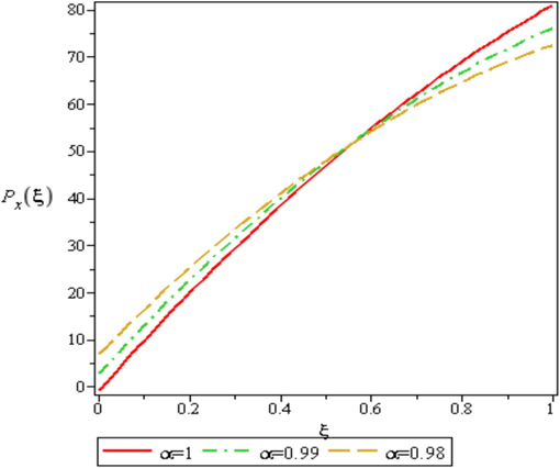
Response of the solution of
at
and
, with parameter:
.
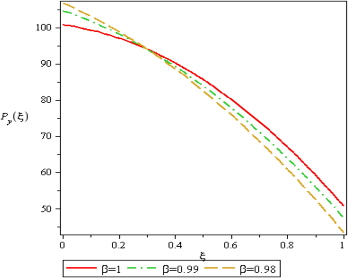
Response of the solution of
at
and
, with parameter:
.
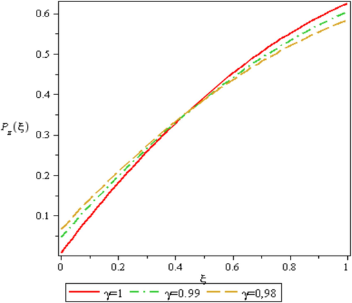
Response of the solution of
at
and
, with parameter:
.
It is evident from these outcomes of the study that the obtained solution regularly changes from fractional order to integer order. From Fig. 1, we observe that the value of increases with increasing time . Decreasing the order of non-integer order derivatives leads to increase in the value of initially, after some time its nature is opposite. From Fig. 2, we notice that the value of decrease with increasing time on . Decreasing the order of arbitrary order derivatives leads to diminution in the value of initially, after some time its nature is opposite. From Fig. 3 we inspect that value of increase with increasing time . On decreasing the order of fractional derivatives leads to an enhancement in the value of initially, after some time its nature is opposite.
It is evident that the results vary continuously from arbitrary order to classical order. Both the exact solution as well as the approximate solutions obtained by using our proposed scheme is presented in the Table 1. We have compared outcomes obtained by Jacobi polynomial, exact solution and method (Singh, 2017; Kumar et al., 2014). Table 1 reveals that the results of the described technique are faithful for practical implementations of FBE.
Pj
ξ
Exact Solution
Present Method
Kumar et al. (2014)
Singh (2017)
Px(ξ)
0.2
19.6693
19.7950
19.6677
19.6528
0.4
38.1707
38.3376
38.1413
38.1798
0.6
54.7955
54.7148
54.6270
54.8107
0.8
68.9228
68.9267
68.3307
68.9246
1
80.0432
80.0292
78.4583
80.0270
Py(ξ)
0.2
97.0315
97.0346
97.0783
97.1108
0.4
90.2823
90.2021
90.3399
90.3047
0.6
80.0943
80.1943
79.8246
80.0340
0.8
66.9388
67.0111
65.5723
66.8616
1
51.3951
51.3826
47.6269
51.3626
Pz(ξ)
0.2
0.1813
0.1802
0.1813
0.1813
0.4
0.3297
0.3285
0.3297
0.3297
0.6
0.4512
0.4520
0.4512
0.4512
0.8
0.5507
0.5508
0.5507
0.5507
1
0.6321
0.6321
0.6321
0.6321
6 Conclusions
In this study, we have suggested a computational scheme for arbitrary order Bloch equation pertaining to the Caputo −Fabrizio operator. The proposed method offers notable advantages in terms of simplicity and user-friendliness compared to alternative techniques, primarily due to the straightforward construction of the operational matrix for differential equations. Specifically, we develop an operational matrix for Caputo-Fabrizio integration by utilizing the Jacobi polynomial. When , we observe strong agreement between the solution obtained through operational matrix techniques and the exact solution of the Bloch equation of arbitrary order. These findings underscore the suitability and accuracy of our proposed approach for analyzing fractional order models employing the Caputo-Fabrizio operator. Future endeavors will delve into the utilization of various special functions such as Bernstein and Vieta Lucas, alongside the operational matrix method, while also exploring the impacts of arbitrary orders on the dynamics of the Bloch equation.
CRediT authorship contribution statement
Jagdev Singh: Writing – review & editing, Supervision, Software, Conceptualization. Jitendra Kumar: Writing – original draft, Software, Methodology, Conceptualization. Dumitru Baleanu: Visualization, Validation, Investigation, Formal analysis.
Declaration of Competing Interest
The authors declare that they have no known competing financial interests or personal relationships that could have appeared to influence the work reported in this paper.
References
- A theoretical basis for the application of fractional calculus to viscoelasticity. J. Rheol.. 1983;27(3):201-210.
- [CrossRef] [Google Scholar]
- Fractional calculus in the transient analysis of viscoelasticity damped structures. American Institute of Aeronautics and Astronautics Journal.. 1985;23:918-925.
- [CrossRef] [Google Scholar]
- A new operational matrix of fractional integration for shifted Jacobi polynomials. Bulletin of the Malaysian Mathematical Sciences Society.. 2014;37(4):983-995.
- [Google Scholar]
- Computational analysis of local fractional LWR model occurring in a fractal vehicular traffic flow. Fractal and Fractional.. 2022;6(8):426.
- [CrossRef] [Google Scholar]
- Forecasting the behavior of fractional order Bloch equations appearing in NMR flow via a hybrid computational technique. Chaos Solitons Fractals. 2022;164:112691
- [CrossRef] [Google Scholar]
- An efficient numerical scheme for fractional model of telegraph equation. Alex. Eng. J.. 2022;61(8):6383-6393.
- [CrossRef] [Google Scholar]
- A general fractional formulation and tracking control for immunogenic tumor dynamics. Mathematical Methods in the Applied Sciences.. 2022;45(2):667-680.
- [CrossRef] [Google Scholar]
- Theory and Applications of Fractional Differential Equations. 2006;Vol. 204:Elsevier.
- A study on eco-epidemiological model with fractional operators. Chaos Solitons Fractals. 2022;156:111697
- [CrossRef] [Google Scholar]
- Fractional calculus in medical and health science. CRC Press; 2020.
- A fractional model of Navier-Stokes equation arising in unsteady flow of a viscous fluid. Journal of the Association of Arab Universities for Basic and Applied Sciences.. 2015;17:14-19.
- [CrossRef] [Google Scholar]
- Computational analysis of local fractional partial differential equations in realm of fractal calculus. Chaos Solitons Fractals. 2023;167:113009
- [CrossRef] [Google Scholar]
- A Fractional model of Bloch equation in nuclear magnetic resonance and its analytic approximate solution. Walailak. J. Sci. Technol.. 2014;11(4):273-285.
- [CrossRef] [Google Scholar]
- A numerical analysis for fractional model of the spread of pests in tea plants. Numer. Methods Partial Differential Equations. 2022;38(3):540-565.
- [CrossRef] [Google Scholar]
- On the attenuation of the perfectly matched layer in electromagnetic scattering problems with the spectral element method. Appl. Comput. Electromagn. Soc. J.. 2014;29(9)
- [Google Scholar]
- Persistence of Photonic Nanojet Formation under the Deformation of Circular the Journal of the Optical Society of America b.. 2016;33(4):535-542.
- [CrossRef]
- On-and off-optical-resonance dynamics of dielectric microcylinders under plane wave illumination. The Journal of the Optical Society of America b.. 2015;32(6):1022-1030.
- [CrossRef] [Google Scholar]
- An introduction to the fractional calculus and fractional differential equations. Wiley; 1993.
- Properties of caputo-fabrizio fractional operators. New Trends in Mathematical Sciences.. 2020;8(1):1-25.
- [CrossRef] [Google Scholar]
- Fractional order modeling the gemini virus in capsicum annuum with optimal control. Fractal and Fractional.. 2022;6(2):61.
- [CrossRef] [Google Scholar]
- The use of control systems analysis in neurophysiology of eye movements. Annu. Rev. Neurosci.. 1981;4:462-503.
- [Google Scholar]
- A new numerical algorithm for fractional model of Bloch equation in nuclear magnetic resonance. Alex. Eng. J.. 2016;55(3):2863-2869.
- [CrossRef] [Google Scholar]
- Operational matrix approach for approximate solution of fractional model of Bloch equation. Journal of King Saud University-Science.. 2017;29(2):235-240.
- [CrossRef] [Google Scholar]
- Analysis of fractional blood alcohol model with composite fractional derivative. Chaos Solitons Fractals. 2020;140:110127
- [CrossRef] [Google Scholar]
- Computational study of fractional order smoking model. Chaos Solitons Fractals. 2021;142:110440
- [CrossRef] [Google Scholar]
- Computational analysis of fractional modified Degasperis-Procesi equation withCaputo-Katugampola derivative. AIMS Mathematics.. 2023;8(1):194-212.
- [CrossRef] [Google Scholar]
- A fractional epidemiological model for computer viruses pertaining to a new fractional derivative. Appl. Math Comput.. 2018;316:504-515.
- [CrossRef] [Google Scholar]
- New trends in fractional differential equations with real-world applications in physics. Frontiers Media SA; 2020.
- New aspects of fractional Bloch model associated with composite fractional derivative. Mathematical Modelling of Natural Phenomena.. 2021;16:10.
- [CrossRef] [Google Scholar]
- On the analysis of an analytical approach for fractional Caudrey-Dodd-Gibbon equations. Alex. Eng. J.. 2022;61(7):5073-5082.
- [CrossRef] [Google Scholar]
- Numerical simulation for fractional-order Bloch equation arising in nuclear magnetic resonance by using the Jacobi polynomials. Appl. Sci.. 2020;10(8):2850.
- [CrossRef] [Google Scholar]
- An application of the Gegenbauer wavelet method for the numerical solution of the fractional Bagley-Torvik equation. Russ. J. Math. Phys.. 2019;26:77-93.
- [CrossRef] [Google Scholar]
- A new numerical investigation of fractional order susceptible-infected-recovered epidemic model of childhood disease. Alex. Eng. J.. 2022;61(2):1747-1756.
- [CrossRef] [Google Scholar]


