

Translate this page into:
Supernonlinear wave, associated analytical solitons, and sensitivity analysis in a two-component Maxwellian plasma
⁎Corresponding author at: Department of Automation, Biomechanics and Mechatronics, Lodz University of Technology, 1/15 Stefanowskiego St., 90-924 Lodz, Poland. bilalsehole@gmail.com (Muhammad Bilal Riaz)
-
Received: ,
Accepted: ,
This article was originally published by Elsevier and was migrated to Scientific Scholar after the change of Publisher.
Peer review under responsibility of King Saud University.
Abstract
This analysis investigates the occurrence of super nonlinear waves in a two-component electron-ion plasma containing Maxwell distributed electrons. The effect of Mach number (M) on the presence of SNWs is also discussed. Analytical findings for all conceivable dark-pitch solitons, singular solitons, associated hyperbolically, trigonometrically, and rational solitons, and super nonlinear periodic wave solutions are discussed in this study. A graphical representation of the research findings is also presented. This study successfully shows 2D- graphs to offer further insight into the physical properties of the solutions described for the various ranges of M that is, for the velocity of the wave profile will be treated as subsonic, for the velocity of the wave profile will be treated as supersonic and for the velocity of the wave profile will be treated as sonic for super nonlinear waves in two-component Maxwellian plasma. We have further demonstrated the sensitivity assessments for the altered dynamical structural system’s supersonic, subsonic, and sonic wave profiles, utilizing six unique initial conditions. That whole research justifies the appearance of SNWs in such a two-component Maxwellian plasma, which used to be formerly unidentified until about the study’s start in 2011. The new analytical findings of the different categories and sensitivity analysis for the dynamical system with supersonic, subsonic, and sonic wave profiles are new things here.
Keywords
Mach number
Supernonlinear waves
Generalized auxiliary equation method
Soliton solutions

1 Introduction
Interestingly, depending on the M, a limited exceed (Das et al., 2012) throughout the magnitude towards a solitary wave was discovered. The researchers, on the other hand, proved powerless to characterize the pattern of a newly discovered form of a solitary wave that differed from nonlinear solitary waves. Dubinov et al. (2012) designated such novel forms of waves as SNWs, which have been characterized by the nontrivial topology of the phase plots, for the very first instance in plasmas. A while back, super nonlinear waves in three-, four, or five components plasma systems were investigated for the small magnitude (Chapagai et al., 2020; Tamang and Saha, 2020) as well as arbitrary amplitude (Taha and El-Taibany, 2020; Saha and Tamang, 2019) limitations. Consequently, three-component Maxwellian or non-Maxwellian plasmas might create super nonlinear solitary and super nonlinear periodic waves in plasmas. If a small amplitude nonlinear wave is considered using the reductive perturbation method and the KdV equation in a two-component electron-ion Maxwellian plasma is obtained, the coefficient of a nonlinear term is 1, i.e. a constant. As a result, higher-order corrections cannot be considered in a two-component electron-ion Maxwellian plasma. Also, in conclusion, small amplitude super nonlinear wave solutions aren’t feasible in a two-component electron-ion Maxwellian plasma. Only solitary and periodic wave solutions are feasible in this instance. In contrast, Cairns et al. (1995) stated where there exists a potential well in its positive direction on a two-component Maxwellian plasma, and therefore there exists a homoclinic loop throughout the phase domain of the differential equation that symbolizes a solitary wave exhibiting positive potential.
In this investigation, we obtained many solutions with the help of generalized auxiliary equation (GAE) method (Akinyemi et al., 2021), for SNWs in Maxwellian plasma with two components (Saha et al., 2020), including hyperbolic trigonometric, trigonometric, exponential, and rational. Therefore the light, darkened, periodic, singular, and exclusive soliton solutions that seem to be truly significant throughout mathematical physics were discovered underneath the variety of restriction constraints. So far as the authors are informed, no previous work on soliton solutions using the GAE technique has been published. An additional advantage of this technique is that it could be applied to other nonlinear models that are connected to it. In fact, the super nonlinear wave (SNW) is characterized by the nontrivial topology of their phase portraits. In this case, the paths contain at least two stable equilibrium points (centers) and one separatrix layer. These waves exist in the plasma system having three or more components. These can be studied by the direct and reductive perturbation techniques. It is good to understand that the phase paths of the dynamical system are the wave solution of the corresponding plasma system (Saha and Banerjee, 2021).
Non-linear differential equations have been commonly used to characterize a comprehensive variety of complex scientific phenomena, such as optics, deeper water, quantum mechanics, biophysics, fluid mechanics, plasma physics, marine engineering, chemistry, as well as physics. However, In literature, the more magnificent technique for finding new exact and explicit solutions for non-linear PDEs (Riaz et al., 2021). Because soliton solutions may be discovered in a variety of mathematical physics models, the theory of optical solitons is highly fascinating. One of the most important elements of nonlinear fiber optics is the observation of optical solitons. Soliton has several applications in applied science and engineering. There are several effective techniques for addressing nonlinear differential equations. Just a few examples include the new extended direct algebraic method (Jhangeer et al., 2020; Munawar et al., 2021; Jhangeer et al., 2021; Hussain et al., 2021; Hussain et al., 2020).
Relying upon the research of Atangana-Baleanu, Abdou et al. (2020) researchers discover novel solutions to the space-time fractional nonlinear Schrödinger equation, where –expansion and generalised Kurdyashov techniques are proposed. Fractional calculus having increasingly piqued the attention of many researchers in domains including physics, plasma physics, nonlinear optics and fractional characteristics, control system, signal processing, biology, architecture, fluid mechanics with visco elasticity, and so on (Abdou, 2017; Manafian, 2016). In Khater et al. (2018), researchers use a novel approach for solving the higher order nonlinear Schrödinger equation, which represents the propagation of brief light pulses in monomode optical fibres. The optical soliton to Wu-Zhang set of evolution equations depicts a (1 + 1)-dimensional dispersive long wave (Jawad and Al Azzawi, 2019). Several organizations in space-time fractional nonlinear optics as well as other fields having researched optical soliton solution in the conclusion (Edeki et al., 2019; Abdou and Yildirim, 2012; Mena-Contla et al., 2018).
Rational sine-Gordon expansion method which is a generalized form of the sine-Gordon expansion method is a newly developed method for analytical solutions (Yel et al., 2022). The generalized variable separation method and the extended homoclinic test the approach is implemented for the construction of the non-traveling wave solutions of -dimensional breaking soliton equation (Shang, 2022). Jhangeer et al. (2021), closely scrutinized the traveling wave solutions of a family of long-wave unstable lubrication models, a study of the perturbed Fokas-Lenells model’s traveling, periodic, quasiperiodic, and chaotic structures, as well as the dynamical analysis and phase pictures of two-mode waves in various mediums. Exact solutions regarding blood flow via a circular tube underneath magnetic field impact employing fractional Caputo-Fabrizio derivatives (Rihan et al., 2016) as well as Synchronization for tumor-immune framework involving fractional-order (Riaz and Zafar, 2018; Jhangeer et al., 2012; Jhangeer, 2018; Jhangeer et al., 2020) were evaluated together a systematic investigation to find and analyze the evidence to determine the reality by M.B. Riaz. Fractional calculus has made a major advancement in the development of solving models for implementations, and it attempts to illustrate that it can create more realistic models, Ghalib et al. (2020), Riaz et al. (2016), Ghalib et al. (2020), Riaz et al. (2020), Riaz et al. (2020), Riaz (2018), and Riaz et al. (2021).
The following is how paper is made: Section 2 is devoted to demonstrating the idea of the proposed method, i.e, GAE method. Section 3, deals with the quest of SNWs in Maxwellian plasma with two components. A simple electron-ion plasma composed of cold mobile ions as well as Maxwell distribution electrons is defined by the dimensionless fundamental equations in the exploration of SNWs. The wave frame is used to transfer the fundamental equations into the nonlinear ordinary differential equation. In Section 4 there is the application of GAE method to find soliton solutions. Furthermore, we have seen various textures of waves in the 2D graphical representation of the solutions, for different values of M. Visualization of study findings in a graphical format is discussed in Section 5. In Section 6, there is the sensitivity assessment for the supersonic, subsonic, and sonic wave profiles. Section 7 deals with the discussions and results analysis. We assessed various dynamic performances, structures, and texturing of wave solutions by analyzing graphs relying on their physical ranges. Associated numerical values for parameters were utilized as an aspect of our investigation to explore distinct dynamic behavior, patterns, and textures of wave solutions. In subSection 7.1 there is a comparative examination of the current study with the previously published literature. Section 8 includes the study’s conclusion.
2 Recapitulation for the GAE method
Throughout this segment, readers analyze the core notion of the GAE methodology (Akinyemi et al., 2021) through investigating the nonlinear PDE of the manner:
Assume Eq. (3) seems to have the following solutions:
Family:1 For
, we have;
Family:2 For
and
, we have;
Family:3 For
and
, we have;
Family:4 For
and
, we have;
Family:5 For
and
, we have;
Family:6 For
and
, we have;
Family:7 For
, we have;
Family:8 For
and
, we have;
Family:9 For
, we have;
Family:10 For
and
, we have;
During which . There are four basic types of solutions: hyperbolic trigonometric, trigonometric, exponential, and rational. However many polynomial equations in of indeterminate variables are gathered into Eqs. (4) and (5) are replaced into Eq. (3) and the coefficients of being equal to zero. Consequently, simply solving the preceding nonlinear polynomial equations, inserting the resulting constants in Eq. (4) with such a known N, and considering the aforementioned solutions set on Eq. (4), we rapidly find the suitable solutions of Eq. (1).
3 The quest of SNWs in Maxwellian plasma with two components
We consider a simple electron-ion plasma composed of cold mobile ions as well as Maxwell distribution electrons defined by the dimensionless fundamental equations in exploration of SNWs (Saha et al., 2020):
n is the number density for ions, along with is the number density for electrons, which is normalized to is the number density for ions at unperturbed condition, along with is the number density for electrons at unperturbed condition. Since, where u is ion’s velocity and is electrostatic potential) is normalized to ion-acoustic speed , where e is electron charge and m is mass of ions. The length of , i.e, and inverse of ion plasma frequency, i.e, is normalized to the space variable i.e, time denoted by .
To analyze supernonlinear and other nonlinear waves in the given plasma system, we use the wave frame below.
When Eqs. (25) and (26) are applied to Eq. (24) and up to third degree terms are included, one may get:
4 Application of GAE method
Within that segment, the GAE method is used to solve Eq. (22). We achieve
, by balancing
and
. As a result, the solution corresponding to Eq. (4) may be written as:
Placing Eqs. (5) as well as (28) inside (22) and setting the coefficient of
to zero yields the foregoing:
When we solve the above equations for the parameters , and , we get the following solutions:
Set 1.
Set 2.
Moreover, the solutions of Eq. (27) are stated as follows, using Eqs. (28) and (30) in relation towards the solution sets established in Section 2:
-
For ,
(32)(33) -
For and ,
(34)(35) -
For and ,
(36)(37) -
For and ,
(38)(39) -
For and ,
(40)(41) -
For and ,
(42)(43) -
For ,
(44) -
For and ,
(45) -
For ,
(46) -
For and ,
(47)Consequently, the solutions for Eq. (27) are stated here as pursues, employing Eqs. (28) and (31) with respect towards the solution sets specified in Section 2:
-
For ,
(48)(49) -
For and ,
(50)(51) -
For and ,
(52)(53) -
For and ,
(54)(55) -
For and ,
(56)(57) -
For and ,
(58)(59) -
For ,
(60) -
For and ,
(61) -
For ,
(62) -
For and ,
(63)
5 Visualization of study findings in a graphical format
This particular phase is devoted to displaying a graphical depiction of a few of the analytical results mentioned throughout this work. The section as a whole reflects on the fundamental understanding of some of the specific outcomes reported in this study. A modern professional programming software application is used to create graphs for better demonstration. Furthermore, each 2D plot is visible over an individual interval. Based on their physical ranges, corresponding numerical values for parameters can be employed. Using varied parameter values as a core component of our experimentation, we may study distinct dynamic characteristics, shapes, and texturing of soliton solutions. It is essential to note, however, that solutions have trigonometric functions, mixed hyperbolic functions, and rational functions.
Fig. 1: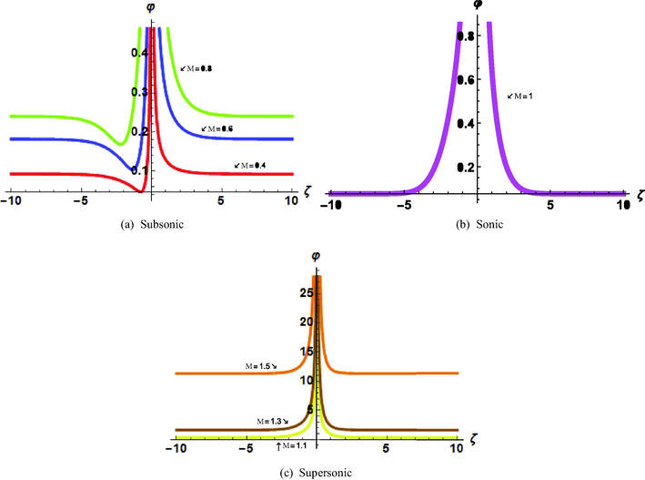
2-dimensional plots of
, for different velocity of the wave profile.
The conclusion of the analysis is established on the proposed parameters’ constant values. The effectiveness of the GAE technique is visually shown as exhibits. Here is a graphic representation of 2D-plot over the interval for different values of M, along with the parameters such as,
, (red), (blue), (green), (magenta), (yellow), (brown), (orange),
Fig. 2: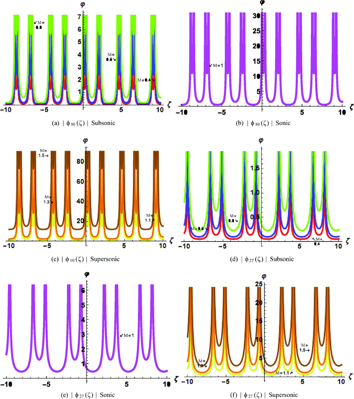
2-dimensional plots for different velocity of the wave profile.
The conclusion of the analysis is established on the proposed parameters’ constant values. The effectiveness of the GAE technique is visually shown as exhibits. Here is a graphic representation of 2D-plot over the interval for different values of M, along with the parameters such as,
, (red), (blue), (green), (magenta), (yellow), (orange), (brown), also the conclusion of the analysis is established on the proposed parameters’ constant values. The effectiveness of the GAE technique is visually shown as exhibited. Here is a graphic representation of 2D-plot over the interval for different values of M, along with the parameters such as,
, (red), (blue), (green), (magenta), (yellow), (orange), (brown),
Fig. 3: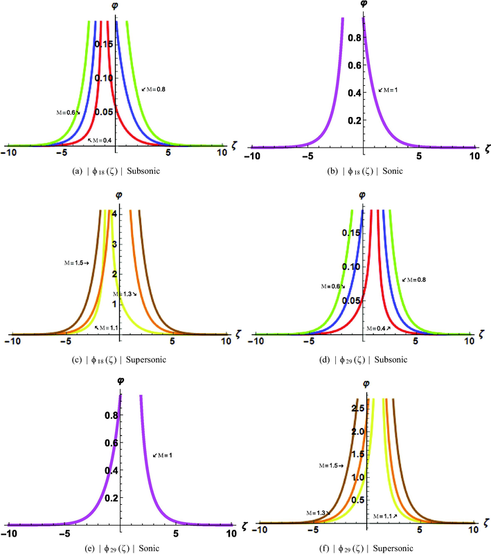
2-dimensional plots for different velocity of the wave profile.
The conclusion of the analysis is established on the proposed parameters’ constant values. The effectiveness of the GAE technique is visually shown as exhibits. Here is a graphic representation of 2D-plot over the interval for different values of M, along with the parameters such as,
, (red), (blue), (green), (magenta), (yellow), (orange), (brown),
Also the conclusion of the analysis is established on the proposed parameters’ constant values. The effectiveness of the GAE technique is visually shown as exhibits. Here is a graphic representation of 2D-plot over the interval for different values of M, along with the parameters such as,
, (red), (blue), (green), (magenta), (yellow), (orange), (brown),
Fig. 4: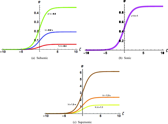
2-dimensional plots of
, for different velocity of the wave profile.
The dark solution, is established on the proposed parameters’ constant values. The effectiveness of the GAE technique is visually shown as exhibits. Here is a graphic representation of 2D-plot over the interval for different values of M, along with the parameters such as,
, (red), (blue), (green), (magenta), (yellow), (orange), (brown),
Fig. 5: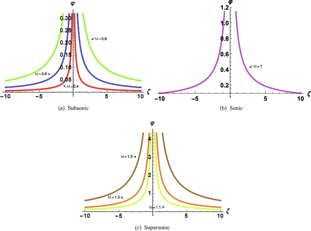
2-dimensional plots of
, for different velocity of the wave profile.
The conclusion of the analysis is established on the proposed parameters’ constant values. The effectiveness of the GAE technique is visually shown as exhibits. Here is a graphic representation of 2D-plot over the interval for different values of M, along with the parameters such as,
, (red), (blue), (green), (magenta), (yellow), (orange), (brown),
Fig. 6: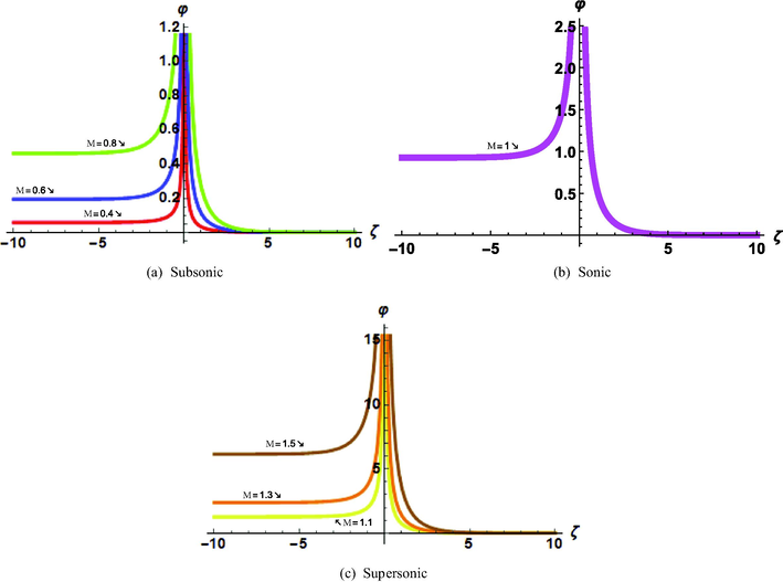
2-dimensional plots of
, for different velocity of the wave profile.
The singular solution, is established on the proposed parameters’ constant values. The effectiveness of the GAE technique is visually shown as exhibits. Here is a graphic representation of 2D-plot over the interval for different values of M, along with the parameters such as,
, (red), (blue), (green), (magenta), (yellow), (orange), (brown),
6 The sensitivity assessment
Eq. (27) can be further represented in the format of a planer dynamical system employing the Galilean transformation as:
We will now look into the sensitive phenomena of the following perturbed system. The mechanism Eq. (27) is subsequently deconstructed in the autonomous conservative dynamical system
as shown below:
Wherein b seems to be the frequency and
is the perturbed term’s strength (Jhangeer et al., 2020). The superficial periodic force is evident in system (65) though not in system (64). To examine Eq. (27)’s sensitive behavior in the existence of a perturbation factor involving the parameters
, and
. Throughout this section, we will look at how the frequency term affects the model under consideration. For this, we will establish the physical characteristics of the investigated model and discuss the influence of the perturbation’s force as well as frequency. Therefore in the segment, we want to know the sensitivity for the solution of the perturbed dynamical structural system (65) by using six distinctive initial conditions:
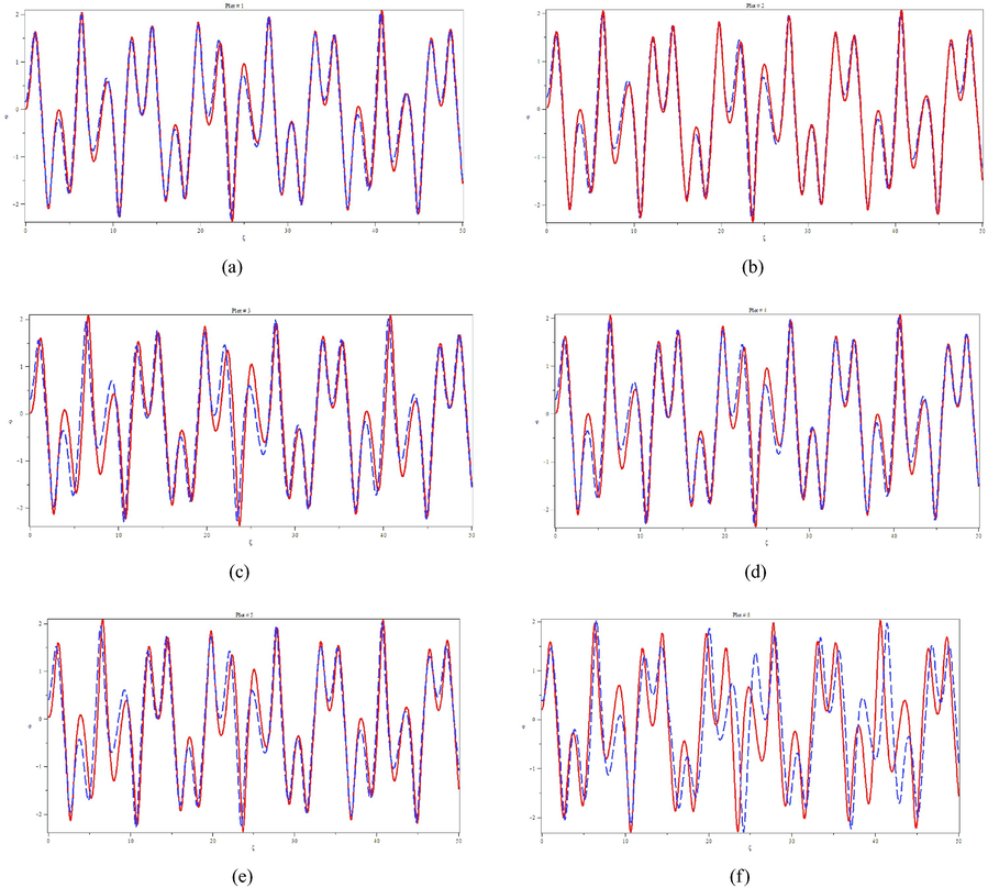
Sensitivity Assessment for Supersonic, Subsonic, and Sonic wave profile
Figure
Red Solid Curve (
)
Dashed Blue line (
)
(a)
(0.00, 0.00)
(0.15, 0.15)
(b)
(0.03, 0.03)
(0.25, 0.25)
(c)
(0.015, 0.015)
(0.30, 0.30)
(d)
(0.02, 0.02)
(0.30, 0.30)
(e)
(0.035, 0.035)
(0.40, 0.40)
(f)
(0.20, 0.20)
(0.40, 0.40)
While the values of the other parameters are the same for each part in Figs. 7–9.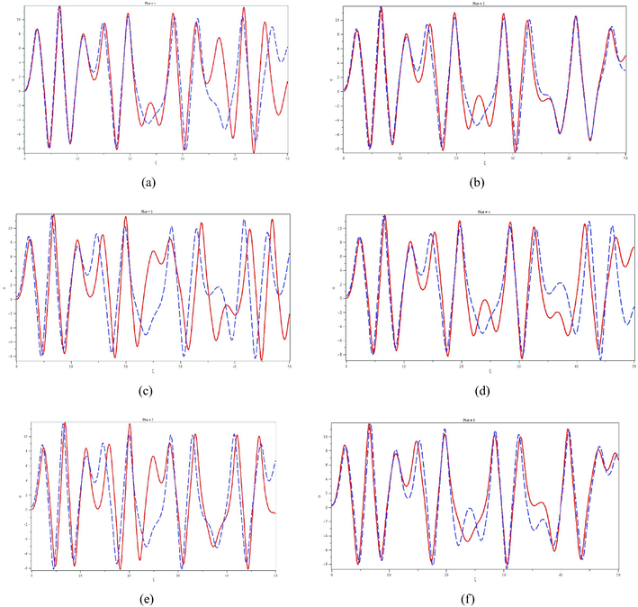
Graphical Representation of Supersonic wave profile for
.
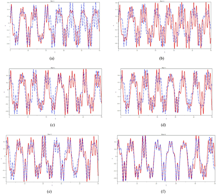
Graphical Representation of Subsonic wave profile for
.
Graphical Representation of Sonic wave profile for
.
A sensitivity assessment is an analysis to know how much our system is sensitive. If there is a minor change in the system by setting minor changes in initial conditions, then the system will have low sensitivity. But, if there is a major change in the system by setting minor changes in initial conditions, then the system will have high sensitivity. In Fig. 9, we can see the sensitivity for the supersonic wave profile for of the perturbed dynamical structural system (65) by using six distinctive initial conditions. For example, in Fig. 7(a), the system is not sensitive from the beginning but as progress from 10 towards 50 in the specified interval, one can observe the change in the amplitude structure of the waves so these curves are not overlapping there, hence the system is sensitive here.
In Fig. 8, we can see the sensitivity for the subsonic wave profile for of the perturbed dynamical structural system (65) by using six distinctive initial conditions as already described in the table above. As an explanation, in Fig. 8(a), the system is conscientiously sensitive from beginning to end (i.e 0 to 50). But in Fig. 8(f), the system is not sensitive for the interval 20 to 40 approximately, as the amplitude structure of the waves is overlapping there, hence the system is not sensitive here.
Fig. 9 depicts the sensitivity for the sonic wave profile of the perturbed dynamical structural system (65) for by employing six unique initial constraints, as given in the table previous paragraph. As an instance, in Fig. 9, the system has very low sensitivity from beginning to end (i.e 0 to 50). But in Fig. 9(c) and (f), the system is conscientiously sensitive for the interval 0 to 40 and 10 to 50 respectively, as the amplitude structure of the waves are not overlapping there, hence the system is sensitive here. In short, the different figures are drawn for the different values of the M and show the sensitiveness of the system. The change in the amplitudes of the waves in the sensitivity plots is the physical justification of the system’s sensitiveness.
7 Discussions and results analysis
When studying the graphical representations of these solutions, our major objective in this part is to show that the newly acquired solutions are more generic and helpful. By selecting appropriate parameters in the Figures, we present several absolute graphs for different values of M. For the velocity of the wave profile will be treated as subsonic. For the velocity of the wave profile will be treated as supersonic. For the velocity of the wave profile will be treated as sonic. We have seen various textures of wave in the 2D graphical representation of the solutions, for different values of M, as we can see in the interval , where the amplitude structures of the wave increase as the value of M increases. As the velocity of the wave profile is changing, the amplitude structure of the wave changes. One can easily observe that as the velocity of the wave profile is subsonic the amplitude structures of the wave are lower than amplitude structures of the wave for sonic and supersonic. In short words, the amplitude of the solutions is very high because it depends on the value of the M. Due to the increase in the value of the M, there is a very high increase in the amplitude of the solutions. Many new precise solutions, including hyperbolic trigonometric, trigonometric, exponential, and rational, are achieved using the GAE approach. The structure of the singular soliton solution is elaborated in Fig. 8, and the dark soliton solution is shown in Fig. 4. These singular solutions are the special types of the soliton solutions in the solitary wave theory. It depends on the type of analytical to be used for the analysis. In this present method, we have implemented the new GAE method for the construction of new soliton solutions. It is the general method for solitary wave solutions. In Figs. 7–9, we can see the sensitivity assessment for the supersonic, subsonic, and sonic wave profile for , and , respectively, of the perturbed dynamical structural system 65 by using six distinctive initial conditions. A sensitivity assessment is an examination that determines how sensitive our system is. If the system undergoes a modest change as a result of slight adjustments in initial circumstances, the system will have weak sensitivity. However, if the system undergoes a significant change as a result of modest changes in the initial circumstances, the system will be very sensitive. These individuals will undoubtedly contribute much to this virtue. In science and engineering, soliton has a wide range of applications.
7.1 A comparative examination
In Dubinov et al. (2012), the topological categorization of similar SNWs has been presented, and an appropriate terminology is offered for them. Numerous instances show that SNWs can occur in the presence of plasma waves with various physical properties, such as electrostatic (ion-acoustic) as well as MHD (Alfvén) waveforms. It is demonstrated that the predominance of at least three separate charged plasma phases is required for the emergence of SNWs. The structure of the SNWs phase image grows increasingly intricate as the quantity of plasma elements grows.
Cairns et al. (1995) stated where there exists a potential well in its positive direction on a two-component Maxwellian plasma, and therefore there exists a homoclinic loop throughout the phase domain of the differential equation that symbolizes a solitary wave exhibiting positive potential. However, for two-component nonthermal plasma that supports both compression as well as rarefactive solitary wave structures for supersonic velocity of the wave profile with (approximately), the cineraria becomes distinct. There was no mention of SNWs.
The occurrence of SNWs in a two-component electron-ion plasma with Maxwell dispersed electrons is investigated in the study (Saha et al., 2020). The influence of M on the presence of SNWs is also discussed. By altering M, phase dynamics are examined using the Hamiltonian function.
While the current study looks on the occurrence of SNWs in a two-component electron-ion plasma with Maxwell distributed electrons. The influence of the M on the presence of SNWs is also addressed. This work highlighted the novel analytical findings of the distinct categories and sensitivity assessment for the dynamical system containing supersonic, subsonic, and sonic wave profiles. Here exists additionally a graphical characterization of the research outcomes.
8 Conclusion
The latest investigation looked at the soliton solutions of a super nonlinear wave in a two-component electron-ion Maxwellian plasma while the velocity of the wave profile is supersonic, sonic, as well as subsonic. The aforementioned nonlinear model is converted into an ordinary differential equation using a wave frame. The GAE methodology is then utilized to produce numerous more exact solutions, such as hyperbolic trigonometric, trigonometric, exponential, but rather rational solutions. Some of the solutions generated can be classified as light, periodic, dark, and even singular solitons. A set of constraint conditions allows for these solutions. In the mentioned figures, we have provided a few two-dimensional plots to highlight the solutions we have developed. We have seen various textures of waves in the 2D graphical representation of the solutions, for different values of M. We also see the sensitivity assessment for the supersonic, subsonic, and sonic wave profile respectively, of the perturbed dynamical structural system by using six distinctive initial conditions. As the velocity of the wave profile is changing, the amplitude structure of the wave changes. A comparative examination of the current study has been done. The proposed research focuses on the occurrence of SNWs in a two-component electron-ion plasma with Maxwell dispersed electrons. The effect of the M on the existence of SNWs is also considered. This paper emphasised the unique analytical findings of the different categories as well as the sensitivity evaluation for the dynamical system encompassing supersonic, subsonic, and sonic wave profiles. The reported results are novel, suggesting that the proposed approach is easy, effective, and applicable to a diverse variety of nonlinear differential equations throughout mathematical physics. It might be emphasized, however, in comparison to prior research work, the interpretations provided in this study are published for the first time.
Declaration of Competing Interest
The authors declare that they have no known competing financial interests or personal relationships that could have appeared to influence the work reported in this paper.
References
- An analytical method for space-time fractional nonlinear differential equations arising in plasma physics. J. Ocean Eng. Sci.. 2017;2(4):288-292.
- [Google Scholar]
- Approximate analytical solution to time fractional nonlinear evolution equations. Int. J. Numer. Methods Heat Fluid Flow 2012
- [Google Scholar]
- Optical soliton solutions for a space-time fractional perturbed nonlinear Schrödinger equation arising in quantum physics. Results Phys.. 2020;16:102895
- [Google Scholar]
- Nonlinear dispersion in parabolic law medium and its optical solitons. Results Phys.. 2021;26:104411
- [Google Scholar]
- Electrostatic solitary structures in non–thermal plasmas. Geophys. Res. Lett.. 1995;22(20):2709-2712.
- [Google Scholar]
- Bifurcation analysis for small-amplitude nonlinear and supernonlinear ion-acoustic waves in a superthermal plasma. Zeitschrift für Naturforschung A. 2020;75(3):183-191.
- [Google Scholar]
- Dust ion-acoustic solitary structures in non-thermal dusty plasma. J. Plasma Phys.. 2012;78(2):149-164.
- [Google Scholar]
- Conformable decomposition for analytical solutions of a time-fractional one-factor markovian model for bond pricing. Appl. Math. Inf. Sci.. 2019;13(4):539-544.
- [Google Scholar]
- Analytical approach for the steady MHD conjugate viscous fluid flow in a porous medium with nonsingular fractional derivative. Phys. A. 2020;554:123941
- [Google Scholar]
- Analytical results on the unsteady rotational flow of fractional-order non-Newtonian fluids with shear stress on the boundary. Discrete Continuous Dyn. Syst.-S. 2020;13(3):683.
- [Google Scholar]
- Optical solitons of fractional complex Ginzburg-Landau equation with conformable, beta, and M-truncated derivatives: a comparative study. Adv. Difference Equ.. 2020;2020(1):1-19.
- [Google Scholar]
- Symmetries, conservation laws and dust acoustic solitons of two-temperature ion in inhomogeneous plasma. Int. J. Geometric Methods Modern Phys.. 2021;18(05):2150071.
- [Google Scholar]
- Soliton Solutions of Wu–Zhang System of Evolution Equations. Numer. Comp. Meth. Sci. Eng.. 2019;1:1-11.
- [Google Scholar]
- Group classification, reductions and exact solutions of a class of higher order nonlinear degenerate parabolic equation. Int. J. Appl. Comput. Math.. 2018;4(1):1-10.
- [Google Scholar]
- Analytic solutions and conserved quantities of wave equation on torus. Comput. Math. Appl.. 2012;64(6):1627-1635.
- [Google Scholar]
- Construction of traveling waves patterns of (1+ n)-dimensional modified Zakharov-Kuznetsov equation in plasma physics. Results Phys.. 2020;19:103330
- [Google Scholar]
- Solitonic, super nonlinear, periodic, quasiperiodic, chaotic waves and conservation laws of modified Zakharov-Kuznetsov equation in transmission line. Commun. Nonlinear Sci. Numer. Simul.. 2020;86:105254
- [Google Scholar]
- Nonlinear self-adjointness, conserved quantities, bifurcation analysis and travelling wave solutions of a family of long-wave unstable lubrication model. Pramana. 2020;94(1):1-9.
- [Google Scholar]
- Analysis of electron acoustic waves interaction in the presence of homogeneous unmagnetized collision-free plasma. Phys. Scr.. 2021;96(7):075603
- [Google Scholar]
- A study of travelling, periodic, quasiperiodic and chaotic structures of perturbed Fokas-Lenells model. Pramana. 2021;95(1):1-11.
- [Google Scholar]
- Dispersive optical soliton solutions for higher order nonlinear Sasa-Satsuma equation in mono mode fibers via new auxiliary equation method. Superlattices Microstruct.. 2018;113:346-358.
- [Google Scholar]
- Optical soliton solutions for Schrödinger type nonlinear evolution equations by the tan (ϕ(ξ)/2))expansion method. Optik. 2016;127(10):4222-4245.
- [Google Scholar]
- Schrödinger solitons in gravitational-like potentials with embedded barriers and wells: Possible applications for the optical soliton supercontinuum generation and the ocean coast line protection. Optik. 2018;159:315-323.
- [Google Scholar]
- New general extended direct algebraic approach for optical solitons of Biswas-Arshed equation through birefringent fibers. Optik. 2021;228:165790
- [Google Scholar]
- Analytical Solutions for Different Motions of Differential and Rate Type Fluids with Fractional Derivatives. Lahore: University of Management of Science; 2018. (Doctoral dissertation)
- Exact solutions for the blood flow through a circular tube under the influence of a magnetic field using fractional Caputo-Fabrizio derivatives. Math. Model. Natural Phenomena. 2018;13(1):8.
- [Google Scholar]
- Analytic solutions of Oldroyd-B fluid with fractional derivatives in a circular duct that applies a constant couple. Alexandria Eng. J.. 2016;55(4):3267-3275.
- [Google Scholar]
- Role of Magnetic field on the Dynamical Analysis of Second Grade Fluid: An Optimal Solution subject to Non-integer Differentiable Operators. J. Appl. Comput. Mech. 2020
- [Google Scholar]
- Computational results with non-singular and non-local kernel flow of viscous fluid in vertical permeable medium with variant temperature. Front. Phys. 2020:275.
- [Google Scholar]
- Nonlinear self-adjointness, conserved vectors, and traveling wave structures for the kinetics of phase separation dependent on ternary alloys in iron (Fe-Cr-Y (Y= Mo, Cu)) Results Phys.. 2021;25:104151
- [Google Scholar]
- Riaz, M.B., Asgir, M., Zafar, A.A. and Yao, S., 2021. Combined Effects of Heat and Mass Transfer on MHD Free Convective Flow of Maxwell Fluid with Variable Temperature and Concentration. Math. Problems Eng..
- Dynamics of tumor-immune system with fractional-order. J. Tumor Res.. 2016;2(1):109-115.
- [Google Scholar]
- Dynamical Systems and Nonlinear Waves in Plasmas. CRC Press; 2021.
- Effect of q-nonextensive hot electrons on bifurcations of nonlinear and supernonlinear ion-acoustic periodic waves. Adv. Space Res.. 2019;63(5):1596-1606.
- [Google Scholar]
- An open problem on supernonlinear waves in a two-component Maxwellian plasma. Eur. Phys. J. Plus. 2020;135(10):1-8.
- [Google Scholar]
- Abundant explicit non-travelling wave solutions for the (2+ 1)-dimensional breaking soliton equation. Appl. Math. Lett. 2022108029
- [Google Scholar]
- Taha, R.M., El-Taibany, W.F., 2020. Bifurcation analysis of nonlinear and supernonlinear dust–acoustic waves in a dusty plasma using the generalized (r, q) distribution function for ions and electrons. Contrib. Plasma Phys. 60(8), p.e202000022.
- Bifurcations of small-amplitude supernonlinear waves of the mKdV and modified Gardner equations in a three-component electron-ion plasma. Phys. Plasmas. 2020;27(1):012105
- [Google Scholar]
- Yel, G., Bulut, H. and lhan, E., 2022. A new analytical method to the conformable chiral nonlinear Schrödinger equation in the quantum Hall effect. Pramana, 96(1), pp.1-11.


