

Translate this page into:
The complex pulsating -Fibonacci sequence
⁎Corresponding author. lkittipo@wu.ac.th (Kittipong Laipaporn)
-
Received: ,
Accepted: ,
This article was originally published by Elsevier and was migrated to Scientific Scholar after the change of Publisher.
Abstract
Several researchers have looked at pulsating Fibonacci sequences in the last ten years, which are generalizations of the Fibonacci sequence. They verify the closed form of these sequences via mathematical induction. This approach is beautiful, but it can only be utilized when patterns of the closed forms are predicted. In this paper, we introduce the complex pulsating -Fibonacci sequence and apply matrix theory, particularly eigenvalues, eigenvectors, and block matrices, as well as basic properties of the floor function to bridge the gap and obtain the closed form of the complex pulsating. Moreover, the golden ratios of this sequence are provided.
Keywords
Pulsating Fibonacci sequence
Golden ratio
Eigenvalue
Eigenvector
Block matrix
The floor function
11B39
11B83
15A21
15A23

1 Introduction and Literature Review
The Fibonacci sequence is defined as and for , and Binet’s formulas for Fibonacci numbers are given by , where , namely, the golden ratio, and . This sequence has been extended in various versions and has also been studied by many mathematicians. For example, Miles (1960) defined the k-generalized Fibonacci numbers by
Horadam (1961) defined the generalized Fibonacci sequence by where p and q are arbitrary integers. Kalman and Mena (2003) generalized the Fibonacci sequence by
Gupta et al. (2012) defined the generalized Fibonacci sequence by
where
and b are positive integers. Wani et al. (2017) defined the generalized k-Fibonacci sequence
by
where q and k are positive integers. Javaheri and Krylov (2020) generalized the Fibonacci sequence by
where P and Q are nonzero integers. However, Atanassov et al. (1985, 2001) defined four 2-Fibonacci sequences as follows:
Atanassov (2013) extended his sequence (1.2) by establishing the
-pulsated Fibonacci sequence, which is defined by
We note that it was sheer coincidence that the sequences in (1.1)-(1.7) were confirmed in their closed form by using mathematical induction.
In this paper, we use matrix theory, especially eigenvalues, eigenvectors and block matrices, and basic properties of the floor function to find the closed form of the Fibonacci sequence that merges (1.6) and (1.7), named the complex pulsating
-Fibonacci sequence. This sequence is defined as follows: Let
and c be real numbers. Then,
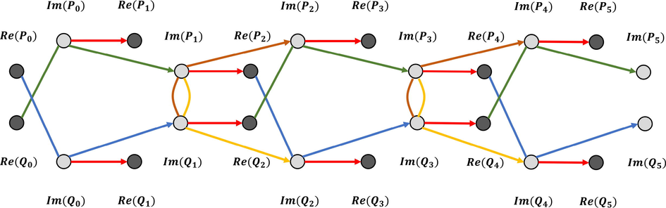
The complex pulsating
-Fibonacci sequence.
Outline of the paper. In Section 2, we give some results which affect the main obtained result. Section 3 is devoted to our main results. The complex pulsating -Fibonacci sequence is given in the closed form. Besides, the golden ratios of this sequence are investigated. Finally, in Section 4, we summarize and discuss our results.
2 Preliminaries
Throughout this paper, let be an m-by-m identity matrix and be an m-by-m matrix in which every entry is one. Let be an m-by-m reversal matrix that is a permutation matrix in which for and all other entries are zero.
In this section, to simplify the process of finding the closed form in Theorem 3.2, we construct the following lemmas.
For any integer , the eigenvalues of matrix are of multiplicity 1, of multiplicity and 1 of multiplicity . Moreover, the eigenvectors of matrix U are
-
with eigenvalue ,
-
with eigenvalue for , where
-
with eigenvalue for , where if m is even, then and if m is odd, then
Obviously, by the properties of the floor function, we have It is easily observed that thus, is the eigenvalue of the matrix U with the corresponding eigenvector .
Next, to show that for all , let and be the ith column of . Then,
Finally, we show that for all . Let and be the ith column of . If m is even, then
If m is odd, then Hence, we have the desired result.
Let U be the matrix which defined in Lemma 2.1 and . Then, when n is even, and when n is odd, where .
By Lemma 2.1, we know that , where P is an m-by-m matrix such that each column vector is an eigenvector of U associated with the eigenvalues and 1 and . To understand the following process more easily, we separate the proof into two cases.
Case 1 If m is odd, then it is easily found that , where . A useful expression for the correspondingly partitioned presentation of m-by-m matrices and is and
We know that and . Let . Then, by carrying out a partitioned multiplication and then simplifying, we write as follows: where
Then, we can rewrite to conclude that if n is even, then , and if n is odd, then .
Case 2 If m is even, then it is easy to see that and , where . By the same argument as in Case 1, we obtain the matrix , where and we can rewrite and hence, if n is even, then , and if n is odd, then , where , as desired.
3 Main results
Two portions are divided in this section. The closed form of the complex pulsating -Fibonacci sequence, which is the focus of the study, is demonstrated in the first section. The golden ratios of this sequence are discussed in the second half.
3.1 The closed form of the complex pulsating -Fibonacci sequence
In this section, matrix theory is an essential proof technique. We will reveal the reasoning behind this choice in Section 4. However, to visualize it more clearly, we would like to provide an example of the following sequence.
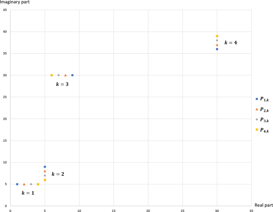
In the circumstances , and , we shall demonstrate an example of the complex pulsating -Fibonacci sequence. Table 1 and Fig. 2 provide more information.
The closed form of the complex pulsating -Fibonacci sequence is for all .
Define a linear transformation
by
Note that U is the matrix in Lemma 2.1. Then, the matrix A can be rewritten in the following form: We are now ready to find the closed form. For each , we let , where and . Moreover, we observe that
. By computing directly, we have where and . Furthermore, by block matrix multiplication, we obtain where and
As a result,
We know that . Next, we let and , and consider the terms of matrix multiplication in two cases:
Case 1 If k is odd, we obtain that and . Thus,
1)
2)
3)
4)
Case 2 If k is even, we obtain that and . In the same manner, we have both and are equal to
. However, and
As a result,
| k | ||||||||
|---|---|---|---|---|---|---|---|---|
| 1 | 1 | 5 | 2 | 5 | 3 | 5 | 4 | 5 |
| 2 | 5 | 9 | 5 | 8 | 5 | 7 | 5 | 6 |
| 3 | 9 | 30 | 8 | 30 | 7 | 30 | 6 | 30 |
| 4 | 30 | 36 | 30 | 37 | 30 | 38 | 30 | 39 |
| 5 | 36 | 150 | 37 | 150 | 38 | 150 | 39 | 150 |
| ⋮ | ⋮ | ⋮ | ⋮ | ⋮ | ⋮ | ⋮ | ⋮ | ⋮ |
- The complex pulsating
-Fibonacci sequence.
3.2 The golden ratio of the complex pulsating -Fibonacci sequence
In mathematics, the Fibonacci sequence and the golden ratio are closely related. This ratio is the limit of the ratios of successive terms of the Fibonacci sequence. In the previous section, we discover the closed form of the complex pulsating -Fibonacci sequence, which is a generalization of the Fibonacci sequence. As a consequence, it is no surprise that we will look at the golden ratio of this sequence in this section. The consequence of our closed form in Section 3.1 is the ratios and which seem to be the well-known golden ratio. For further results, look at the following proposition.
For each , let be a complex pulsating -Fibonacci sequence as the sequence (1.8). Then, the golden ratios of this sequence are
-
,
-
.
First, for each , we consider the ratio by using Theorem 3.2 and in the same manner, we have
As a result, . In addition, by the same argument, we obtain for all . So, we have
And,
4 Conclusion and Discussion
Actually, the heart of this paper is to find the appropriate matrix Q to use in the proof of Theorem 3.2 but the matrix Q can take many different forms. The variety of Q depends on a linear map T which obeys the rule in (1.8). Here is one of the examples of Q that we ever used to solve (1.8). Let for and be defined by where . Then the matrix Q is in the form where In the same manner, we know that , where , . The matrix looks uneasily to compute its closed form. So, here is the reason that we choose the map T in (3.1) because its matrix representation is in the form which is easily compute . Even though, the matrix looks so complicated but it can be decomposed as follows: . Moreover, the matrix is the inverse of , which makes it easier to see . Then, the computation of is simplified to only find the matrix . So, we have to collect all of the eigenvalues and eigenvectors in Lemma 2.1 and complete our work in Lemma2.2 for finding the closed form of . Until now, we can see that the construction of Q relies on the rearrangement in the entries of the matrix and the formula of a map T. Both of these may lead us to vary directions for getting Q.
By the way, we believe that our tactics to create the matrix Q in Section 3.1 are not the best. So, we wish to see a friendly matrix Q that can be computed favorably.
Acknowledgment
We would like to thank the reviewers for their valuable suggestions. This research was financially supported by Walailak University Grant No. WU63247 and the new strategic research project (P2P) fiscal year 2022, Walailak University, Thailand.
Declaration of Competing Interest
The authors declare that they have no known competing financial interests or personal relationships that could have appeared to influence the work reported in this paper.
References
- A new perspective to the generalization of the Fibonacci sequence. Fibonacci Quart.. 1985;23:21-28.
- [Google Scholar]
- New visual perspectives on Fibonacci numbers. Singapore: World Scientific Publishing; 2001. pp. 3–38
- Complete generalized Fibonacci sequences modulo primes. Mosc. J. Comb. Number Theory. 2020;9:1-15.
- [Google Scholar]
- Generalized Fibonacci numbers and associated matrices. Amer. Math. Monthly. 1960;67:745-752.
- [Google Scholar]


