

Translate this page into:
A new one-parameter discrete exponential distribution: Properties, inference, and applications to COVID-19 data
⁎Corresponding authors. ahmed.afify@fcom.bu.edu.eg (Ahmed Z. Afify), hector.gomez@uantof.cl (Héctor W. Gómez)
-
Received: ,
Accepted: ,
This article was originally published by Elsevier and was migrated to Scientific Scholar after the change of Publisher.
Peer review under responsibility of King Saud University.
Abstract
A new one-parameter discrete length-biased exponential distribution called the discrete moment exponential (DMEx) distribution is introduced using the survival discretizing approach. We derive the reliability measures including survival function, hazard function, residual reliability function, and the second rate of failure function. Further, the mathematical properties of the DMEx distribution are derived. The parameters of the DMEx distribution are estimated using seven estimation methods. A simulation study is carried out to explore the behavior of the proposed estimators. It is observed that the maximum likelihood approach provides efficient estimates. Finally, the DMEx is adopted for fitting the number of COVID-19 deaths in China and Europe countries. It is shown that the DMEx distribution fits the data better than other competing discrete distributions.
Keywords
Discretization method
Simulation
Statistical inference
Data analysis
COVID-19

1 Introduction
In the last decades, several discrete distributions have been introduced as analogs of the continuous distributions to have a better alternative model for modeling count data sets having complicated behavior. Although classical models such as binomial, Poisson, Geometric, and negative binomial distributions are used to model count data sets, in some situations, these probability models do not provide the best fit. Hence there is a need to develop more flexible distributions.
Several discretization methods have been adopted extensively in the literature to define new discrete models. Chakraborty (Chakraborty, 2015) conducted a survey on several discretization methods available to derive discrete analogs of continuous distributions, such as discretization methods based on survival function (SF), probability density function (PDF), cumulative distribution function (CDF), hazard rate function (HRF), reversed-HRF, the difference equation analog of Persian differential equation and a two-stage composite method.
Let a random variable (rv)
follows a continuous probability distribution with SF
. Using the SF discretization method which is introduced by Kemp (2004), the probability mass function (PMF) of a discrete rv is specified by.
Using this method of discretization several discrete distribution have been introduced, such as the discrete Weibull (Nakagawa and Osaki, 1975), discrete Rayleigh (Roy, 2004), discrete half-normal (Kemp, 2008), discrete Burr and discrete Pareto (Krishna and Singh Pundir, 2009), discrete inverse-Weibull (Jazi et al., 2010), generalized geometric (Gómez-Déniz, 2010), discrete Lindley (Gomez-Deniz and Calderin-Ojeda, 2011), generalized exponential type II (Nekoukhou et al., 2013), two-parameter discrete Lindley (Hussain et al., 2016), new discrete extended-Weibull (Jia et al., 2019), natural discrete-Lindley (Al-Babtain et al., 2020); discrete MO-Weibull (Opone et al., 2020), uniform Poisson–Ailamujia (Aljohani et al., 2021), discrete inverted Topp-Leone (Eldeeb et al., 2021), discrete power-Ailamujia (Alghamdi et al., 2022), Binomial-exponential 2 (Bakouch et al., 2017), Poisson-exponential (Rodrigues et al., 2018), and discrete Ramos-Louzada (Ramos and Louzada, 2019; Afify et al., 2021).
Dara and Ahmad (2012) introduced the moment-exponential (MEx) distribution and showed that it is more flexible than the exponential distribution. The PDF of MEx distribution is specified by.
The corresponding SF has the form
Using the discretization method based on the SF, a discrete analog of continuous MEx distribution is introduced in this paper.
In this article, we propose the asymmetric discrete distribution called the discrete moment exponential (DMEx) distribution using the discretization method based on SF. The DMEx distribution is a competitor to some well-known discrete models such as the discrete Burr, discrete Burr-Hatke, discrete Rayleigh, discrete inverted Topp-Leon, discrete Pareto, discrete inverse Rayleigh, and Poisson distributions. The parameter of the DMEx model is estimated using seven classical estimation approaches. We present the detailed simulation results to address the behavior of the estimators.
The rest of this paper is outlined six sections. In Section 2, we define the new DMEx distribution and provide some of its basic properties. The estimation approaches are presented in Section 3. The efficiency of the introduced estimators is assessed via simulation results in Section 4. Section 5 provides two real applications to COVID-19 data of the DMEx distribution. Section 6 presents some final conclusions.
2 The DMEx distribution and its properties
The DMEx distribution is obtained using Eqs. (1) and (3). The PMF of the DMEx distribution has the form (for
)
The corresponding CDF of the DMEx model reduces to
Fig. 1 shows the PMF behavior of the DMEx distribution for different values of
. It is observed that the DMEs PMF has unimodal behavior and positively skewed for
. The mode of the DMEx distribution moves towards the left for large values of
.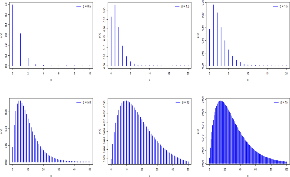
The PMF plots of the DMEx distribution.
2.1 Survival, hazard rate, and quantile functions
The SF of the DMEx distribution reduces to
The HRF of the DMEx distribution takes the form
Fig. 2 shows that the behavior of the HRF of the DMEx model is increasing for different values of
.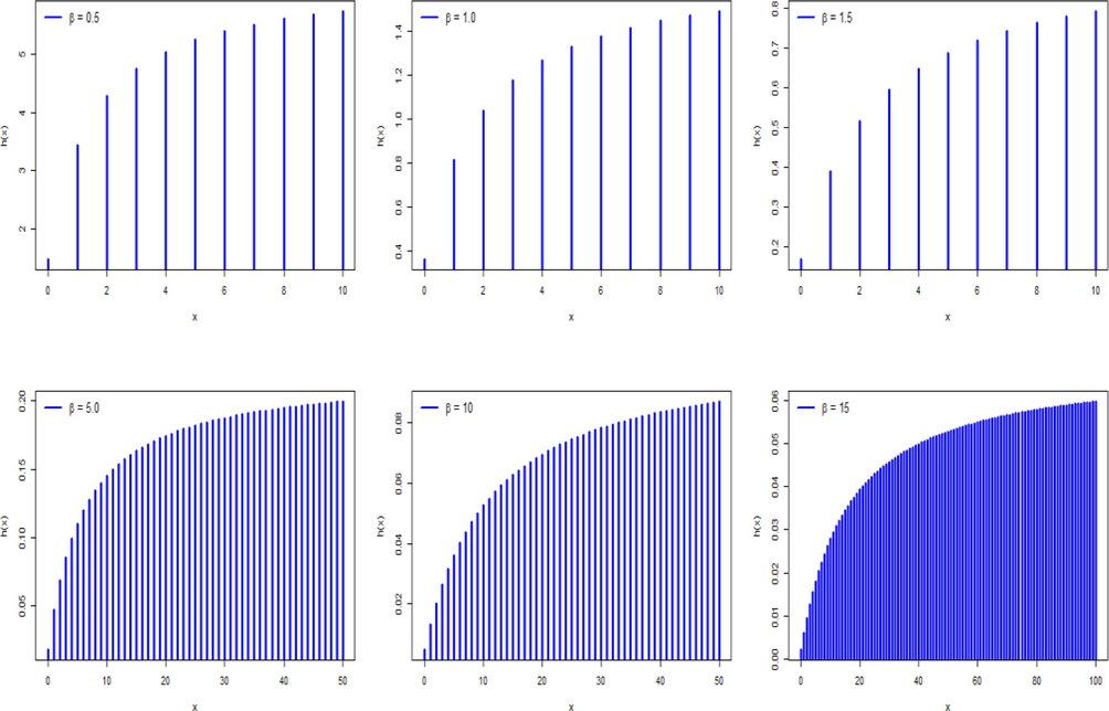
The HRF plots of the DMEx distribution.
The second rate of failure, say , of the DMEs model is defined as.
The reversed HRF of the DMEx distribution is
The quantile function (QF) of the DMEx model takes the form where is the integer part of and is the negative branch of the Lambert function.
2.2 Probability generating function and moments
The probability generating function of the DMEx distribution follows as
Differentiating with respect to and setting , we can obtain the first four factorial moments of the DMEx distribution as follows
The first four ordinary moments of the DMEx distribution can be calculated using the factorial moments as follows
The variance of the DMEx distribution has the form
Further, the coefficient of skewness and kurtosis of the DMEx distribution can be calculated by the formulae and
2.3 Dispersion index
The index of dispersion (DI) is defined as
The DI shows that whether a distribution is suitable for modeling under-dispersed data or over-dispersed data. The distribution is over-dispersed for
and for
it is under-dispersed. Table 1 reports some numerical values for the descriptive measures of the DMEx distribution. Table 1 shows that the DMEs model is useful for both over-dispersed and under-dispersed data sets. The DMEx also exhibits positively skewed which supported by the plots of its PMF in Fig. 1.
Parameter
Descriptive Measures
β
Mean
Variance
Skewness
Kurtosis
DI
0.2
0.0409
0.0403
4.8256
25.763
0.9839
0.5
0.5185
0.5253
1.5011
11.266
1.0130
0.8
1.1050
1.3364
1.3678
18.932
1.2093
1.0
1.5027
2.0653
1.3668
23.323
1.3745
1.5
2.5008
4.5750
1.3838
31.074
1.8294
2.0
3.5003
8.0786
1.3950
35.852
2.3079
2.5
4.5002
12.580
1.4013
39.022
2.7955
3.0
5.5001
18.081
1.4049
41.263
3.2874
4.0
7.5000
32.082
1.4089
44.209
4.2776
5.0
9.5000
50.083
1.4108
46.052
5.2718
9.0
17.500
162.08
1.4131
49.473
9.2618
3 Parameter estimation
In this section, we estimate the parameter of the DMEx distribution using seven methods of estimation.
3.1 Maximum likelihood (ML)
Suppose be a random sample of size from the DMEx distribution. Then, the log-likelihood function reduces to
The ML estimator (MLE) of follows by solving that is
The MLE of cannot be calculated explicitly. Hence, numerical methods can be adopted to obtain it.
3.2 Methods of Anderson-Darling and right-tail Anderson-Darling
Let be the th order statistic in a sample of size . The Anderson-Darling (AD) test is proposed by (Anderson and Darling, 1952). Let be the AD estimator (ADE) which is obtained by minimizing the following equation
This estimator of
can also be derived by solving
where
and it reduces to
The right-tail Anderson-Darling (RADE) of the parameter follows by minimizing
The RADE is also calculated by solving
3.3 Method of Cramèr-von-Misses
Macdonald (Macdonald, 1971) proved that the Cramèr-von-Mises estimator (CVME) has a smaller bias as compared to other minimum distance type estimators. The CVME of follows by minimizing
The CVME of is also obtained by solving
3.4 Methods of least-squares and weighted least-squares
The least-squares estimator (LSE) of follows by minimizing with respect to . Moreover, the LSE of is also obtained by solving
The weighted least-squares estimator (WLSE) of follows by minimizing
The WLSE of can also be obtained by solving
In which is presented in (6).
3.5 Methods of percentiles
Suppose that is an unbiased estimator of . Hence, the percentiles estimator (PCE) (Kao, 1959) of the parameter can be derived by minimizing the following equation where is the negative branch of the Lambert function.
4 Simulation study
Here we conduct a Monte Carlo simulation study to compare the performance of different methods of estimation. The performance of different estimators is evaluated based on mean square errors (MSEs), mean relative errors (MREs) and average absolute biases (ABBs) which are given by. and
The introduced methods are compared for sample sizes,
=5, 10, 30, 50, and 100. To this end, we generate 10,000 independent samples of size
from the DMEx distribution with different values of
= 0.5, 1.0, 2.0, 3.0, 5.0 and 9.0. It is observed that 10,000 repetitions are sufficiently large enough to have stable results. The results of the simulations are reported in Tables 2–4.
Measure
MLE
LSE
WLE
PCE
CVME
ADE
RADE
10
AABs
0.0588
0.3887
0.4145
0.2315
0.3888
0.3826
0.3710
25
0.0169
0.3879
0.4427
0.2022
0.3878
0.3792
0.3678
50
0.0032
0.3874
0.4650
0.1888
0.3874
0.3797
0.3665
100
0.0012
0.3878
0.4838
0.1808
0.3877
0.3791
0.3662
150
0.0007
0.3870
0.4945
0.1777
0.3876
0.3792
0.3656
200
0.0009
0.3872
0.5022
0.1752
0.3875
0.3790
0.3656
10
MREs
0.2354
1.5546
1.6581
0.9259
1.5551
1.5305
1.4840
25
0.0677
1.5518
1.7708
0.8087
1.5511
1.5168
1.4712
50
0.0128
1.5497
1.8601
0.7551
1.5497
1.5189
1.4659
100
0.0047
1.5511
1.9350
0.7232
1.5507
1.5166
1.4649
150
0.0029
1.5481
1.9780
0.7106
1.5503
1.5166
1.4624
200
0.0037
1.5488
2.0088
0.7008
1.5501
1.5159
1.4624
10
MSEs
0.0198
0.1530
0.1756
0.0586
0.1531
0.1480
0.1386
25
0.0058
0.1512
0.1980
0.0430
0.1511
0.1443
0.1356
50
0.0014
0.1505
0.2172
0.0366
0.1505
0.1445
0.1344
100
0.0006
0.1506
0.2345
0.0332
0.1505
0.1439
0.1342
150
0.0004
0.1499
0.2449
0.0319
0.1503
0.1439
0.1337
200
0.0003
0.1500
0.2526
0.0309
0.1503
0.1437
0.1337
10
AABs
0.0051
0.3368
0.3715
0.2471
0.3371
0.3290
0.2983
25
0.0004
0.3306
0.3995
0.2117
0.3313
0.3224
0.2888
50
0.0011
0.3311
0.4241
0.1940
0.3294
0.3197
0.2864
100
0.0010
0.3290
0.4484
0.1835
0.3295
0.3189
0.2848
150
0.0001
0.3289
0.4633
0.1783
0.3289
0.3180
0.2841
200
0.0000
0.3285
0.4745
0.1758
0.3290
0.3181
0.2834
10
MREs
0.0103
0.6735
0.7429
0.4941
0.6741
0.6579
0.5966
25
0.0007
0.6611
0.7989
0.4234
0.6627
0.6448
0.5777
50
0.0022
0.6622
0.8482
0.3881
0.6587
0.6395
0.5729
100
0.0019
0.6580
0.8967
0.3670
0.6590
0.6377
0.5696
150
0.0002
0.6578
0.9266
0.3567
0.6578
0.6361
0.5682
200
0.0001
0.6570
0.9490
0.3517
0.6580
0.6362
0.5667
10
MSEs
0.0161
0.1271
0.1492
0.0795
0.1268
0.1222
0.1014
25
0.0058
0.1145
0.1639
0.0515
0.1149
0.1094
0.0885
50
0.0030
0.1123
0.1821
0.0409
0.1111
0.1048
0.0844
100
0.0015
0.1095
0.2022
0.0353
0.1098
0.1030
0.0823
150
0.0010
0.1090
0.2155
0.0329
0.1090
0.1020
0.0815
200
0.0007
0.1086
0.2258
0.0317
0.1089
0.1019
0.0809
Measure
MLE
LSE
WLE
PCE
CVME
ADE
RADE
10
AABs
0.0088
0.3362
0.3488
0.2921
0.3359
0.3348
0.2916
25
0.0011
0.3259
0.3496
0.2346
0.3230
0.3182
0.2750
50
0.0016
0.3197
0.3672
0.2140
0.3159
0.3099
0.2673
100
0.0009
0.3171
0.3847
0.1951
0.3185
0.3116
0.2643
150
0.0008
0.3154
0.3986
0.1884
0.3145
0.3074
0.2645
200
0.0001
0.3152
0.4066
0.1848
0.3146
0.3074
0.2620
10
MREs
0.0088
0.3362
0.3488
0.2921
0.3359
0.3348
0.2916
25
0.0011
0.3259
0.3496
0.2346
0.3230
0.3182
0.2750
50
0.0016
0.3197
0.3672
0.2140
0.3159
0.3099
0.2673
100
0.0009
0.3171
0.3847
0.1951
0.3185
0.3116
0.2643
150
0.0008
0.3154
0.3986
0.1884
0.3145
0.3074
0.2645
200
0.0001
0.3152
0.4066
0.1848
0.3146
0.3074
0.2620
10
MSEs
0.0502
0.1755
0.1768
0.1498
0.1740
0.1708
0.1388
25
0.0201
0.1305
0.1429
0.0799
0.1274
0.1233
0.0959
50
0.0105
0.1143
0.1442
0.0583
0.1116
0.1074
0.0819
100
0.0052
0.1065
0.1521
0.0439
0.1073
0.1028
0.0751
150
0.0035
0.1034
0.1617
0.0395
0.1028
0.0983
0.0734
200
0.0026
0.1023
0.1674
0.0372
0.1021
0.0975
0.0711
10
AABs
0.0038
0.3618
0.3741
0.3855
0.3511
0.3566
0.3139
25
0.0047
0.3243
0.3399
0.2932
0.3221
0.3216
0.2730
50
0.0011
0.3231
0.3428
0.2427
0.3222
0.3187
0.2674
100
0.0002
0.3194
0.3410
0.2201
0.3149
0.3103
0.2583
150
0.0002
0.3167
0.3449
0.2017
0.3136
0.3092
0.2558
200
0.0019
0.3115
0.3472
0.1960
0.3129
0.3081
0.2524
10
MREs
0.0019
0.1809
0.1870
0.1928
0.1756
0.1783
0.1570
25
0.0023
0.1621
0.1700
0.1466
0.1611
0.1608
0.1365
50
0.0005
0.1616
0.1714
0.1213
0.1611
0.1594
0.1337
100
0.0001
0.1597
0.1705
0.1100
0.1575
0.1552
0.1292
150
0.0001
0.1583
0.1724
0.1009
0.1568
0.1546
0.1279
200
0.0010
0.1557
0.1736
0.0980
0.1565
0.1541
0.1262
10
MSEs
0.1982
0.3722
0.3850
0.4017
0.3602
0.3516
0.3187
25
0.0782
0.1980
0.2090
0.1805
0.1976
0.1920
0.1568
50
0.0411
0.1524
0.1615
0.1069
0.1519
0.1470
0.1141
100
0.0201
0.1253
0.1374
0.0720
0.1223
0.1181
0.0876
150
0.0134
0.1160
0.1330
0.0560
0.1142
0.1106
0.0793
200
0.0099
0.1083
0.1306
0.0506
0.1097
0.1061
0.0741
Measure
MLE
LSE
WLE
PCE
CVME
ADE
RADE
10
AABs
0.0130
0.3975
0.4179
0.4705
0.3643
0.3769
0.3574
25
0.0014
0.3498
0.3519
0.3383
0.3386
0.3420
0.2850
50
0.0097
0.3335
0.3295
0.2823
0.3243
0.3245
0.2559
100
0.0003
0.3206
0.3306
0.2340
0.3168
0.3147
0.2509
150
0.0060
0.3175
0.3288
0.2218
0.3119
0.3100
0.2496
200
0.0037
0.3126
0.3289
0.2095
0.3114
0.3088
0.2447
10
MREs
0.0043
0.1325
0.1393
0.1568
0.1214
0.1256
0.1191
25
0.0005
0.1166
0.1173
0.1128
0.1129
0.1140
0.0950
50
0.0032
0.1112
0.1098
0.0941
0.1081
0.1082
0.0853
100
0.0001
0.1069
0.1102
0.0780
0.1056
0.1049
0.0836
150
0.0020
0.1058
0.1096
0.0739
0.1040
0.1033
0.0832
200
0.0012
0.1042
0.1096
0.0698
0.1038
0.1029
0.0816
10
MSEs
0.4482
0.7108
0.7379
0.7991
0.6734
0.6494
0.6324
25
0.1827
0.3402
0.3251
0.3305
0.3274
0.3155
0.2765
50
0.0859
0.2208
0.2068
0.1883
0.2129
0.2063
0.1631
100
0.0451
0.1558
0.1590
0.1079
0.1534
0.1489
0.1090
150
0.0305
0.1364
0.1401
0.0846
0.1327
0.1292
0.0942
200
0.0224
0.1234
0.1315
0.0704
0.1239
0.1207
0.0843
10
AABs
0.0021
0.4191
0.4318
0.6349
0.4216
0.4438
0.4216
25
0.0078
0.3448
0.3654
0.4577
0.3491
0.3573
0.3168
50
0.0023
0.3268
0.3433
0.3487
0.3228
0.3296
0.2746
100
0.0055
0.3230
0.3229
0.2768
0.3258
0.3271
0.2530
150
0.0065
0.3100
0.3224
0.2542
0.3174
0.3185
0.2508
200
0.0034
0.3117
0.3252
0.2326
0.3125
0.3136
0.2456
10
MREs
0.0004
0.0838
0.0864
0.1270
0.0843
0.0888
0.0843
25
0.0016
0.0690
0.0731
0.0915
0.0698
0.0715
0.0634
50
0.0005
0.0654
0.0687
0.0697
0.0646
0.0659
0.0549
100
0.0011
0.0646
0.0646
0.0554
0.0652
0.0654
0.0506
150
0.0013
0.0620
0.0645
0.0508
0.0635
0.0637
0.0502
200
0.0007
0.0623
0.0650
0.0465
0.0625
0.0627
0.0491
10
MSEs
1.2552
1.7171
1.6830
1.9589
1.6687
1.5782
1.5649
25
0.5255
0.7323
0.6971
0.8212
0.7176
0.6809
0.6329
50
0.2565
0.3988
0.4034
0.4206
0.4080
0.3907
0.3376
100
0.1213
0.2504
0.2401
0.2277
0.2486
0.2397
0.1982
150
0.0823
0.1969
0.1925
0.1614
0.1990
0.1928
0.1522
200
0.0632
0.1707
0.1734
0.1287
0.1757
0.1708
0.1238
The following conclusions are drawn from Tables 2–4.
-
All the considered estimation methods have consistency property, i.e., the MSEs and MREs decrease with the increasing of the sample size .
-
It is observed that the ML method performs better based on the MSEs as compared to other estimation methods.
5 Applications to COVID-19 data
The flexibility of the DMEx distribution is illustrated using two real-life COVID-19 data sets.
The first data refers to the number of COVID-19 daily deaths in China from 23 January to 28 March (https://www.worldometers.info/coronavirus/country/china/). The observations are listed below in ascending order.
3
3
4
5
5
6
6
7
7
7
8
8
9
10
11
11
13
3
14
15
16
17
22
22
24
26
26
27
28
29
30
31
31
35
38
38
42
43
44
45
46
47
52
57
64
65
71
73
73
86
89
97
97
97
98
105
108
109
114
118
121
136
142
143
146
150
6
18
28
29
44
47
55
116
118
129
150
184
219
236
237
336
421
434
612
648
706
838
1129
1393
1540
1941
2175
2278
2667
2803
2824
n
Min.
Mean
Median
Var
Skewness
Kurtosis
DI
Q3
Max.
Data I
3
49.74
33
1924.8
0.8365
2.4502
38.696
83
150
Data II
6
818.0
336
868739.6
1.0167
2.6308
1062.1
1407
2824
The fitting performance of the DMEx distribution is compared with the following discrete distributions:
-
Discrete Burr (DBurr) distribution. Its PMF is
-
Discrete Burr-Hatke (DBH) distribution. Its PMF is
-
Discrete Rayleigh (DR) distribution. Its PMF is
-
Discrete inverted Topp-Leon (DITL) distribution. Its PMF is
-
Discrete Pareto (DPr) distribution. Its PMF is
-
Discrete inverse Rayleigh (DIR) distribution. Its PMF is
-
Poisson distribution. Its PMF is
The R package called “fitdistrplus” is used to obtain the results in this section. The parameters of the four distributions are estimated using the ML approach. For model comparison, we have considered the log-likelihood (LogL), Akaike’s information criterion (AIC), and Bayesian information criterion (BIC).
The estimates of the parameters and their standard errors (SE) along with goodness of fit measures are presented in Table 6 for both data sets. The values in these tables illustrate that the DMEx provides an adequate fit to the data as compared with other models.
Model
Estimate (SE)
logL
AIC
BIC
Data 1: Number of deaths in China
DMEx
−330.515
663.031
665.220
DBur
−374.500
753.001
757.380
DBH
−461.020
924.039
926.229
DR
−347.227
696.455
698.644
DITL
−366.907
735.815
738.005
DPr
−379.070
760.140
762.330
DIR
−376.380
754.760
756.950
Poisson
−1409.78
2821.57
2823.75
Data 2: Number of deaths in Europe
DMEx
−257.122
516.243
517.677
DBur
−62.902
529.804
532.672
DBH
−56.308
714.616
716.050
DR
−72.816
547.634
549.068
DITL
−59.617
521.234
522.668
DPr
−63.363
528.727
530.161
DIR
−26.987
655.975
657.409
Poisson
−5361.1
30724.2
30725.7
Furthermore, the estimated CDF, SF, and HRF of the DMEx distribution are depicted in Figs. 3(a) and 4(a) for number of deaths in China and Europe, respectively. The probability–probability (P-P) plots of the fitted discrete distributions are displayed in Fisg. 3(b) and 4(b) for the two datasets, respectively.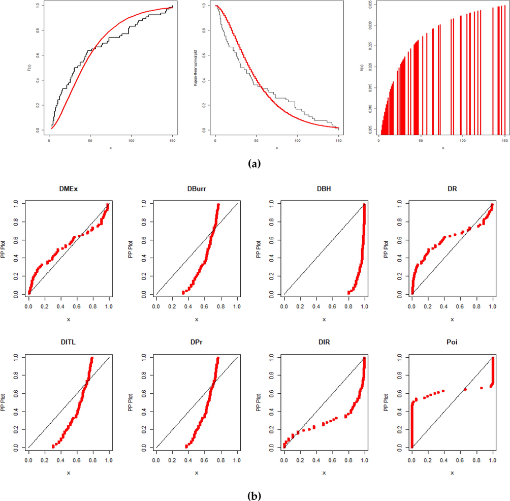
(a) The fitted CDF, SF, and HRF plots of the DMEx model and (b) the P-P plots of the DMEx model and its competing discrete distributions for number of deaths in China.
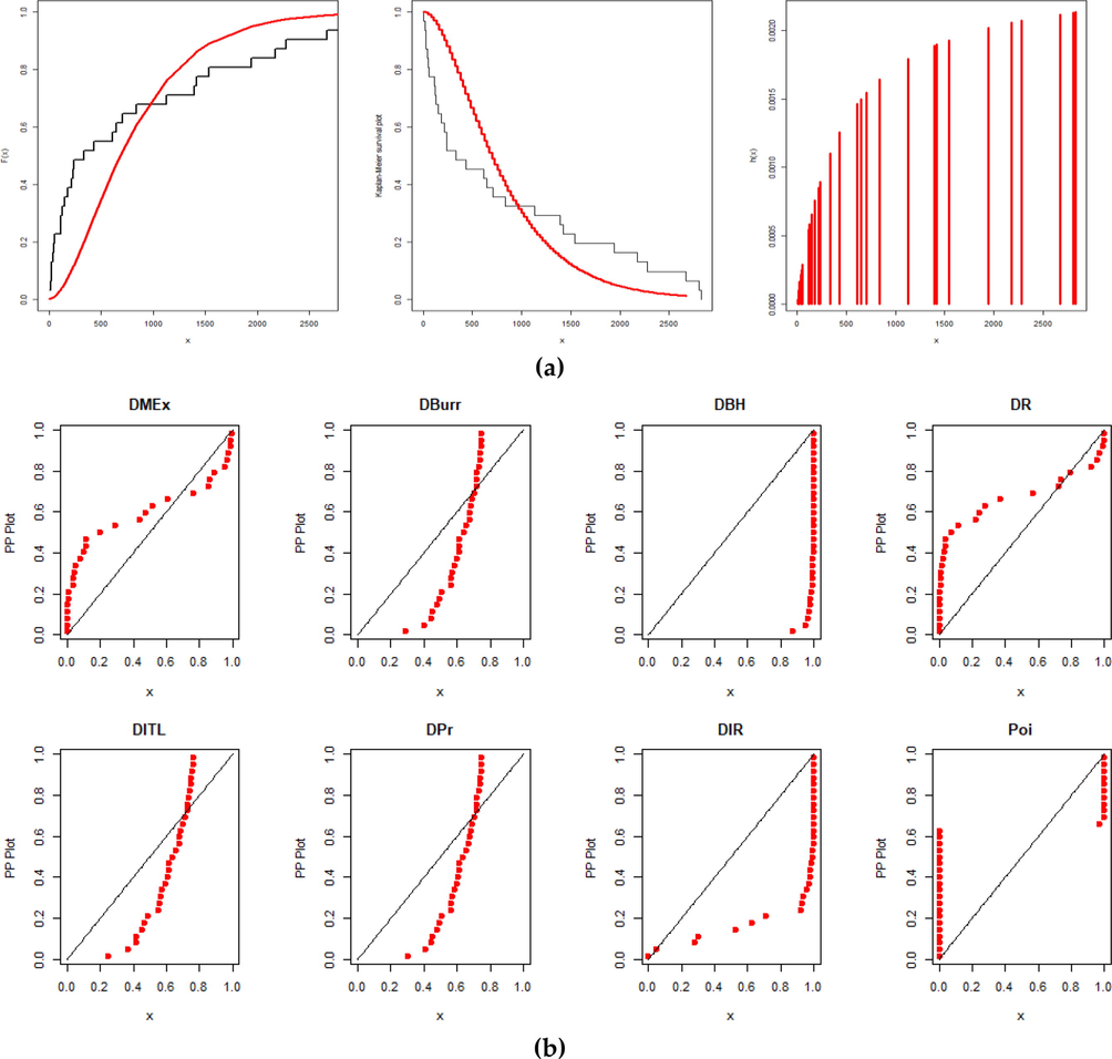
(a) The fitted CDF, SF, and HRF plots of the DMEx model and (b) the P-P plots of the DMEx model and its competing discrete distributions for number of deaths in Europe.
In the two applications, we can indicate that the best model representing the daily deaths by COVID-19 is the DMEx distribution. Based on the fitted model, we can answer some questions such as the probability of having more than deaths per day, whereas a prediction based on the mean to the deaths per day by COVID-19.
6 Conclusion
In this article, a new discrete probability distribution called the discrete moment-exponential (DMEx) distribution is proposed. It can be used as an alternative to some well-known discrete distributions. Its mathematical properties of the DMEx distribution are presented. The model parameters are estimated using seven different estimation methods. Comprehensive simulation results are carried out to compare these methods. Based on our study, the maximum likelihood is recommended to estimate the DMEx parameter. The usefulness of the DMEx distribution is illustrated empirically using two applications to the number of deaths due to COVID-19 in China and Europe. The DMEx distribution is quite competitive to the discrete Burr, discrete Burr-Hatke, discrete Rayleigh, discrete inverted Topp-Leon, discrete-Pareto, discrete inverse-Rayleigh, and Poisson distributions. We hope that the DMEx distribution can be applied to traumatic brain injury data following the paper of Ramos et al. (2019).
Acknowledgement
This study was funded by Taif University Researchers Supporting Project number (TURSP-2020/279), Taif University, Taif, Saudi Arabia.
Declaration of Competing Interest
The authors declare that they have no known competing financial interests or personal relationships that could have appeared to influence the work reported in this paper.
References
- A new skewed discrete model: properties, inference, and applications. Pakistan J. Stat. Oper. Res.. 2021;17:799-816.
- [Google Scholar]
- A new discrete analog of the continuous Lindley distribution, with reliability applications. Entropy. 2020;22:603.
- [Google Scholar]
- The discrete power-Ailamujia distribution: properties, inference, and applications. AIMS Math.. 2022;7:8344-8360.
- [Google Scholar]
- The uniform Poisson-Ailamujia distribution: actuarial measures and applications in biological science. Symmetry. 2021;13:1258.
- [Google Scholar]
- Asymptotic theory of certain“ goodness of fit” criteria based on stochastic processes. Ann. Math. Stat.. 1952;23:193-212.
- [Google Scholar]
- Binomial-exponential 2 distribution: different estimation methods with weather applications. TEMA (São Carlos). 2017;2017(18):233-251.
- [Google Scholar]
- Generating discrete analogues of continuous probability distributions- a survey of methods and constructions. J. Stat. Distrib. Appl.. 2015;2:1-30.
- [Google Scholar]
- Recent advances in Moment distribution and their hazard rates. Lap Lambert academic Publishing GmbH KG; 2012.
- A discrete analog of inverted Topp-Leone distribution: properties, estimation and applications. Int. J. Anal. Appl.. 2021;19:695-708.
- [Google Scholar]
- The discrete Lindley distribution: properties and application. J. Stat. Comput. Simul.. 2011;81:1405-1416.
- [Google Scholar]
- A two parameter discrete Lindley distribution. Revista Colom.Estadistica. 2016;39:45-61.
- [Google Scholar]
- A discrete inverse Weibull distribution and estimation of its parameters. Stat. Methodol.. 2010;7:121-132.
- [Google Scholar]
- A graphical estimation of mixed Weibull parameters in life testing electron tube. Technometrics. 1959;1:389-407.
- [Google Scholar]
- A classes of discrete lifetime distributions. Commun. Stat. Theory Methods. 2004;33(12):3069-3093.
- [Google Scholar]
- Discrete Burr and discrete Pareto distributions. Stat. Methodol.. 2009;6(2):177-188.
- [Google Scholar]
- Comment on “an estimation procedure for mixtures of distributions” by Choi and Bulgren. J. R. Stat. Soc. Ser. B Methodol.. 1971;33:326-329.
- [Google Scholar]
- Discrete generalized exponential distribution of a second type. Statistics. 2013;47:876-887.
- [Google Scholar]
- A Discrete analogue of the continuous Marshall-Olkin Weibull distribution with application to count data. Earthline J. Math. Sci.. 2020;5:415-428.
- [Google Scholar]
- Modeling traumatic brain injury lifetime data: improved estimators for the generalized gamma distribution under small samples. PLoS ONE. 2019;14(8):e0221332.
- [Google Scholar]
- Poisson–exponential distribution: different methods of estimation. J. Appl. Stat.. 2018;45(1):128-144.
- [Google Scholar]


