Dynamical behaviour of shallow water waves and solitary wave solutions of the Dullin-Gottwald-Holm dynamical system

M.H. Raddadi; M. Younis; Aly R. Seadawy; S.U. Rehman; M. Bilal; S.T.R. Rizvi; Ali Althobaiti

doi:10.1016/j.jksus.2021.101627

Dynamical behaviour of shallow water waves and solitary wave solutions of the Dullin-Gottwald-Holm dynamical system

M.H. Raddadi^{^a}, M. Younis^{^b}, Aly R. Seadawy^{^a,⁎}, S.U. Rehman^{^a}, M. Bilal^{^a}, S.T.R. Rizvi^{^c}, Ali Althobaiti^{^d}

a Mathematics Department, Faculty of Science, Taibah University, Al-Madinah Al-Munawarah, Saudi Arabia

b Department of Computer Science, University of the Punjab, Lahore 54000, Pakistan

c Department of Mathematics, COMSATS University Islamabad, Lahore Campus, Lahore, Pakistan

d Department of Mathematics, College of Science, Taif University, P.O. Box 11099, Taif 21944, Saudi Arabia

⁎Corresponding author. aly742001@yahoo.com (Aly R. Seadawy)

Received: 2021-3-3, Accepted: 2021-9-22,

Disclaimer:
This article was originally published by Elsevier and was migrated to Scientific Scholar after the change of Publisher.

Peer review under responsibility of King Saud University.

Abstract

In this article, we recover a variety of new families of shallow water wave and solitary wave solutions to the (1+1)-dimensional Dullin “Gottwald” Holm (DGH) system by employing new extended direct algebraic method (NEDAM). The derived results are obtained in diverse hyperbolic and periodic function forms. The attained solutions are new addition in the study of solitary wave and shallow water wave theory. In addition, 3-dimensional, 2-dimensional, and contour graphs of secured results are plotted in order to observe their dynamics with the choices of involved parameters. On the basis of achieved outcomes, we may claim that the proposed computational method is direct, dynamics, well organized, and will be useful for solving the more complicated nonlinear problems in diverse areas together with symbolic computations.

Keywords

Shallow water waves

Solitary water waves

(1+1)-Dimensional DGH system

NEDAM

Integrability

Show Related Articles from PubMed

1 Introduction

Due to the swift development of symbolic computation software systems, the construction of analytic (exact) solutions of nonlinear partial differential equations (NLPDEs) has a very prominent place in the research of some nonlinear intricate phenomena comprehensively (Bhatti et al., 2020; Cao et al., 2021; Khan et al., 2019; Marin et al., 2020; Seadawy et al., 2020; Seadawy et al., 2020 ). The forms of solutions of NLPDEs, that are combined employing several mathematical norms, are very substantial different sciences such as plasma physics, ocean engineering, fluid dynamics, biophysics, mathematical physics, chemistry, optical fiber,telecommunication, quantum field theory, and many others (Chen, 2020; Iqbal et al., 2018, 2020; Yang et al., 2020; Younis et al., 2020 ). In the recent past, many mathematician and researchers have established several efficient and powerful methodologies to retrieve exact solutions in the forms of traveling wave or solitary wave such as, Lie symmetry analysis, extended rational sine–cosine/ sinh-cosh schemes (Rehman and Ahmad, 2020), extended auxiliary equation method (Rezazadeh et al., 2019), $(\frac{G^{'}}{G^{2}}$ )-expansion function method (Bilal et al., 2020), the extended fan sub-equation technique (Younis et al., 2020), F-expansion function method (Seadawy et al., 2020), Bernoulli sub-equation function method (Syam, 2019), $\exp (- ϕ (ξ))$ -expansion function method (Abdou, 2019), the new generalized rational function method (GERFM) (Younas et al., 2021), ansatz approach, new $Φ^{6}$ -model expansion scheme (Rehman et al., 2020), Lie symmetries (Olver, 2000; Bluman et al., 2009), extended direct algebraic method and its modified form (Çelik et al., 2021; Seadawy et al., 2018), extended mapping method and Seadawy techniques (Khater et al., 2000; Seadawy, 2017; Seadawy et al., 2018 ) and several others (Ancol et al., 2015; da Silva and Freire, 2020; da Silva and Freire, 2019; Younas et al., 2020 ) were established for nonlinear physical models (El-Hameed, 2020). In this studies, (1+1)-dimensional Dullin-Gottwald-Holm (DGH) system is considered and analyzed analytically by deploying new extended direct algebraic method. It shows the unidirectional propagation of surface waves in a shallow water regime. Therefore, it is imperative to examine this considered model analytically and derive the solutions. The DGH system is read as (Dullin et al., 2001),

(1)

ψ_{t} + c_{0} ψ_{x} - α^{2} (ψ_{xxt} + ψ ψ_{xxx} + 2 ψ_{x} ψ_{xx}) + 3 ψ ψ_{x} + γ ψ_{xxx} = 0, t > 0,

where fluid velocity is denoted by

ψ (x, t)

in spatial direction x.

α^{2} (α > 0)

and

\frac{c_{0}}{γ}

represent squares of length scales, where as

c_{0} = \sqrt{gh} (where c_{0} = 2 ω)

denotes the linear wave speed for disturbed water at rest at spatial infinity. In this work, we will implement a mathematical technique NEDAM that will reveal a bunch of exact solutions (Mirhosseni-Alizamini et al., 2020). We note that the studied model has not yet been examined utilizing the NEDAM. NEDAM is one of the robust method to look for the exact solutions of NLPDEs. The layout of the article is arranged in the following order: Analysis of NEDAM is presented in Section 2. Exact solutions are revealed in Section 3. Results and discussion are displayed in Section 4. The concluding remarks are given in last Section 5.

2 Analysis of NEDAM

A detail description is given below.

Step 1: NLPDE is defined in general form as follows:

(2)

Δ (φ, φ_{t}, φ_{tt}, φ_{x}, φ_{xx}, \dots) = 0,

where

Δ

and

φ

represent a polynomial and unknown function respectively.

Step 2:

The variable $η$ is defined to convert two variables x and t in a single form using the following compound transformation.

(3)

φ (x, t) = H (η), η = x - ct,

On solving Eqs. (3) and (2), following ODE is obtained

(4)

Π (H, H^{'}, H^{″}, H^{‴}, \dots) = 0,

where

Π

is a polynomial in H and its derivatives.

Step 3:

Consider the solutions of Eq. (4) in form of $ϒ (η)$ is written as

(5)

H (η) = \sum_{i = 0}^{n} b_{i} ϒ^{i} (η), b_{n} \neq 0,

where

b_{i}

(0 ⩽ i ⩽ n)

are unknown and

ϒ (η)

satisfies the following nonlinear ODE,

(6)

ϒ^{'} (η) = \ln (B) (μ + λ ϒ (η) + ν ϒ^{2} (η)), B \neq 0, 1 .

Further, Eq. (6) has the general solution.

(1) For $λ^{2} - 4 μ ν < 0$ and $ν \neq 0$ , there are five solutions,

(7)

ϒ_{1} (η) = - \frac{λ}{2 ν} + \frac{\sqrt{- (λ^{2} - 4 μ ν)}}{2 ν} \tan_{B} (\frac{\sqrt{- (λ^{2} - 4 μ ν)}}{2} η),

(8)

ϒ_{2} (η) = - \frac{λ}{2 ν} - \frac{\sqrt{- (λ^{2} - 4 μ ν)}}{2 ν} \cot_{B} (\frac{\sqrt{- (λ^{2} - 4 μ ν)}}{2} η),

(9)

ϒ_{3} (η) = - \frac{λ}{2 ν} + \frac{\sqrt{- (λ^{2} - 4 μ ν)}}{2 ν} (\tan_{B} (\sqrt{- (λ^{2} - 4 μ ν)} η) \pm \sqrt{pq} \sec_{B} (\sqrt{- (λ^{2} - 4 μ ν)} η)),

(10)

ϒ_{4} (η) = - \frac{λ}{2 ν} - \frac{\sqrt{- (λ^{2} - 4 μ ν)}}{2 ν} (\cot_{B} (\sqrt{- (λ^{2} - 4 μ ν)} η) \pm \sqrt{pq} \csc_{B} (\sqrt{- (λ^{2} - 4 μ ν)} η)),

(11)

ϒ_{5} (η) = - \frac{λ}{2 ν} + \frac{\sqrt{- (λ^{2} - 4 μ ν)}}{4 ν} (\tan_{B} (\frac{\sqrt{- (λ^{2} - 4 μ ν)}}{4} η) - \cot_{B} (\frac{\sqrt{- (λ^{2} - 4 μ ν)}}{4} η)) .

(2) For $λ^{2} - 4 μ ν > 0$ and $ν \neq 0$ , there are five solutions,

(12)

ϒ_{6} (η) = - \frac{λ}{2 ν} - \frac{\sqrt{λ^{2} - 4 μ ν}}{2 ν} \tanh_{B} (\frac{\sqrt{λ^{2} - 4 μ ν}}{2} η),

(13)

ϒ_{7} (η) = - \frac{λ}{2 ν} - \frac{\sqrt{λ^{2} - 4 μ ν}}{2 ν} \coth_{B} (\frac{\sqrt{λ^{2} - 4 μ ν}}{2} η),

(14)

ϒ_{8} (η) = - \frac{λ}{2 ν} - \frac{\sqrt{λ^{2} - 4 μ ν}}{2 ν} (\tanh_{B} (\sqrt{λ^{2} - 4 μ ν} η) \pm i \sqrt{pq} {sech}_{B} (\sqrt{λ^{2} - 4 μ ν} η)),

(15)

ϒ_{9} (η) = - \frac{λ}{2 ν} - \frac{\sqrt{- (λ^{2} - 4 μ ν)}}{2 ν} (\coth_{B} (\sqrt{λ^{2} - 4 μ ν} η) \pm \sqrt{pq} {csch}_{B} (\sqrt{λ^{2} - 4 μ ν} η)),

(16)

ϒ_{10} (η) = - \frac{λ}{2 ν} + \frac{\sqrt{- (λ^{2} - 4 μ ν)}}{4 ν} (\tanh_{B} (\frac{\sqrt{λ^{2} - 4 μ ν}}{4} η) + \coth_{B} (\frac{\sqrt{λ^{2} - 4 μ ν}}{4} η)) .

(3) For $μ ν > 0$ and $λ = 0$ , there are five solutions,

(17)

ϒ_{11} (η) = \sqrt{\frac{μ}{ν}} \tan_{B} (\sqrt{μ ν} η),

(18)

ϒ_{12} (η) = - \sqrt{\frac{μ}{ν}} \cot_{B} (\sqrt{μ ν} η),

(19)

ϒ_{13} (η) = \sqrt{\frac{μ}{ν}} (\tan_{B} (2 \sqrt{μ ν} η) \pm \sqrt{pq} \sec_{B} (2 \sqrt{μ ν} η)),

(20)

ϒ_{14} (η) = - \sqrt{\frac{μ}{ν}} (\cot_{B} (2 \sqrt{μ ν} η) \pm \sqrt{pq} \csc_{B} (2 \sqrt{μ ν} η)),

(21)

ϒ_{15} (η) = \frac{1}{2} \sqrt{\frac{μ}{ν}} (\tan_{B} (\frac{\sqrt{μ ν}}{2} η) - \cot_{B} (\frac{\sqrt{μ ν}}{2} η)) .

(4) For $μ ν < 0$ and $λ = 0$ , there are five solutions,

(22)

ϒ_{16} (η) = - \sqrt{- \frac{μ}{ν}} \tanh_{B} (\sqrt{- μ ν} η),

(23)

ϒ_{17} (η) = - \sqrt{- \frac{μ}{ν}} \coth_{B} (\sqrt{- μ ν} η),

(24)

ϒ_{18} (η) = - \sqrt{- \frac{μ}{ν}} (\tanh_{B} (2 \sqrt{- μ ν} η) \pm i \sqrt{pq} {sech}_{B} (2 \sqrt{- μ ν} η)),

(25)

ϒ_{19} (η) = - \sqrt{- \frac{μ}{ν}} (\coth_{B} (2 \sqrt{- μ ν} η) \pm \sqrt{pq} {csch}_{B} (2 \sqrt{- μ ν} η)),

(26)

ϒ_{20} (η) = - \frac{1}{2} \sqrt{- \frac{μ}{ν}} (\tanh_{B} (\frac{\sqrt{- μ ν}}{2} η) - \coth_{B} (\frac{\sqrt{- μ ν}}{2} η)) .

(5) For $λ = 0$ and $ν = μ$ , there are five solutions,

(27)

ϒ_{21} (η) = \tan_{B} (μ η),

(28)

ϒ_{22} (η) = - \cot_{B} (μ η),

(29)

ϒ_{23} (η) = \tan_{B} (2 μ η) \pm \sqrt{pq} \sec_{B} (2 μ η),

(30)

ϒ_{24} (η) = - \cot_{B} (2 μ η) \pm \sqrt{pq} \csc_{B} (2 μ η),

(31)

ϒ_{25} (η) = \frac{1}{2} (\tan_{B} (\frac{μ}{2} η) - \cot_{B} (\frac{μ}{2} η)) .

(6) For $λ = 0$ and $ν = - μ$ , there are five solutions,

(32)

ϒ_{26} (η) = - \tanh_{B} (μ η),

(33)

ϒ_{27} (η) = - \coth_{B} (μ η),

(34)

ϒ_{28} (η) = - \tanh_{B} (2 μ η) \pm i \sqrt{pq} {sech}_{B} (2 μ η),

(35)

ϒ_{29} (η) = - \coth_{B} (2 μ η) \pm \sqrt{pq} {csch}_{B} (2 μ η),

(36)

ϒ_{30} (η) = - \frac{1}{2} (\tanh_{B} (\frac{μ}{2} η) + \coth_{B} (\frac{μ}{2} η)) .

(7) For $λ^{2} = 4 μ ν$ , there is one solution,

(37)

ϒ_{31} (η) = \frac{- 2 μ (λ η \ln B + 2)}{λ^{2} η \ln B} .

(8) For $λ = χ, μ = r χ (r \neq 0)$ and $ν = 0$ , there is one solution,

(38)

ϒ_{32} (η) = B^{χ η} - r .

(9) For $λ = ν = 0$ , there is one solution,

(39)

ϒ_{33} (η) = μ η \ln B .

(10) For $λ = μ = 0$ , there is one solution,

(40)

ϒ_{34} (η) = \frac{- 1}{ν η \ln B} .

(11) For $μ = 0$ and $λ \neq 0$ , there are two solutions,

(41)

ϒ_{35} (η) = - \frac{p λ}{ν (\cosh_{B} (λ η) - \sinh_{B} (λ η) + p)},

(42)

ϒ_{36} (η) = - \frac{λ (\sinh_{B} (λ η) + \cosh_{B} (λ η))}{ν (\sinh_{B} (λ η) + \cosh_{B} (λ η) + q)},

(12) For $λ = χ, ν = r χ (r \neq 0)$ and $μ = 0$ , there is one solution,

(43)

ϒ_{37} (η) = \frac{{pB}^{χ η}}{p - {rqB}^{χ η}} .

In the above solutions, the generalized hyperbolic and trigonometric functions are defined as the following citegroup cite36,

\sinh_{B} (η) = \frac{{pB}^{η} - {qB}^{- η}}{2}, \cosh_{B} (η) = \frac{{pB}^{η} + {qB}^{- η}}{2},

\tanh_{B} (η) = \frac{{pB}^{η} - {qB}^{- η}}{{pB}^{η} + {qB}^{- η}}, \coth_{B} (η) = \frac{{pB}^{η} + {qB}^{- η}}{{pB}^{η} - {qB}^{- η}},

{sech}_{B} (η) = \frac{2}{{pB}^{η} + {qB}^{- η}}, {csch}_{B} (η) = \frac{2}{{pB}^{η} - {qB}^{- η}},

\sin_{B} (η) = \frac{{pB}^{i η} - {qB}^{- i η}}{2}, \cos_{B} (η) = \frac{{pB}^{i η} + {qB}^{- i η}}{2},

\tan_{B} (η) = - i \frac{{pB}^{i η} - {qB}^{- i η}}{{pB}^{i η} + {qB}^{- i η}}, \cot_{B} (η) = i \frac{{pB}^{i η} + {qB}^{- i η}}{{pB}^{i η} - {qB}^{- i η}},

\sec_{B} (η) = \frac{2}{{pB}^{i η} + {qB}^{- i η}}, \csc_{B} (η) = \frac{2 i}{{pB}^{i η} - {qB}^{- i η}},

where

η

is an independent variable and

p, q > 0

Step 4:

The N can be calculated using Eq. (4). For this reason, the homogeneous balancing principle is useful in equating the nonlinear terms in Eq. (4) with higher derivatives.

Step 5:

The unknown constants can be obtained by substituting Eq. (5) into Eq. (4) and equating the coefficients of $ϒ (η)$ of similar power to zero, we achieve a set of algebraic expressions. On solving these equations through symbolic computation, we obtain sets of solution.

3 Exact solutions

In order to resolve the governing model by employing NEDAM, we operate the wave transformation $φ (x, t)$ = $H (η), where η = x - ct$ and $c \neq 0$ . Substituting the given transformation into Eq. (1),

(44)

α^{2} {cH}^{‴} - {cH}^{'} + c_{0} H^{'} - α^{2} {HH}^{‴} + γ H^{‴} + 3 {HH}^{'} - 2 α^{2} H^{'} H ″ = 0,

where

'

represent derivative w.r.t

η

Integrating Eq. (44) one time w.r.t $η$ and let the constant of integration equal to 0, turns into following

(45)

H^{″} (α^{2} (- c) - γ + α^{2} H) - (c_{0} - c) H - \frac{3 H^{2}}{2} + \frac{1}{2} α^{2} {(H^{'})}^{2} = 0 .

By making balance between in Eq. (45), yields,

n = 2

. So, the nontrivial Eq. (45) transforms into following

(46)

H (η) = b_{0} + b_{1} ϒ (η) + b_{2} ϒ^{2} (η) .

Putting Eq. (46) along its derivatives in Eq. (45) making the coefficients of similar powers of

ϒ (η)

to 0, we achieve a system of algebraic equations. On solving these equations through symbolic computation, we seek clusters of solutions sets as follows

Family-1. $\{b_{0} = - 4 γ μ ν \ln^{2} (B), b_{1} = - 4 γ λ ν \ln^{2} (B), b_{2} = - 4 γ ν^{2} \ln^{2} (B), α = 0, c_{0} = c - γ \ln^{2} (B) (λ^{2} - 4 μ ν) .\}$ The emerging solutions of Eq. (1) are given in detail as

(1) For $λ^{2} - 4 μ ν < 0$ and $ν \neq 0$ ,

The trigonometric solutions

(47)

ψ_{1} (x, t) = \{γ \ln^{2} (B) (λ^{2} - 4 μ ν) (\tan_{B} {(\frac{1}{2} η \sqrt{4 μ ν - λ^{2}})}^{2} + 1)\} .

(48)

ψ_{2} (x, t) = \{γ \ln^{2} (B) (λ^{2} - 4 μ ν) (\cot_{B} {(\frac{1}{2} η \sqrt{4 μ ν - λ^{2}})}^{2} + 1)\} .

The combo-trigonometric solutions

(49)

ψ_{3} (x, t) = \{γ \ln^{2} (B) (λ^{2} - 4 μ ν) ({(\tan_{B} (η \sqrt{4 μ ν - λ^{2}}) \pm \sqrt{pq} \sec_{B} (η \sqrt{4 μ ν - λ^{2}}))}^{2} + 1)\} .

(50)

ψ_{4} (x, t) = \{γ \ln^{2} (B) (λ^{2} - 4 μ ν) ({(\cot_{B} (η \sqrt{4 μ ν - λ^{2}}) \pm \sqrt{pq} \csc_{B} (η \sqrt{4 μ ν - λ^{2}}))}^{2} + 1)\} .

(51)

ψ_{5} (x, t) = \{\frac{1}{4} γ \ln^{2} (B) (λ^{2} - 4 μ ν) ({(\cot_{B} (\frac{1}{4} η \sqrt{4 μ ν - λ^{2}}) - \tan_{B} (\frac{1}{4} η \sqrt{4 μ ν - λ^{2}}))}^{2} + 4)\} .

(2) For $λ^{2} - 4 μ ν > 0$ and $ν \neq 0$ , various exact solutions are constructed.

The kink solution

(52)

ψ_{6} (x, t) = {- γ \ln^{2} (B) (λ^{2} - 4 μ ν) (\tanh_{B} {(\frac{1}{2} η \sqrt{λ^{2} - 4 μ ν})}^{2} - 1)}

The singular solution

(53)

ψ_{7} (x, t) = \{- γ \ln^{2} (B) (λ^{2} - 4 μ ν) (\coth_{B} {(\frac{1}{2} η \sqrt{λ^{2} - 4 μ ν})}^{2} - 1)\} .

The complex kink-antikink solution

(54)

ψ_{8} (x, t) = \{- γ \ln^{2} (B) (λ^{2} - 4 μ ν) (- 1 + {(\tanh_{B} (η \sqrt{λ^{2} - 4 μ ν}) \pm i \sqrt{pq} {sech}_{B} (η \sqrt{λ^{2} - 4 μ ν}))}^{2})\} .

The mixed singular solution

(55)

ψ_{9} (x, t) = \{- γ \ln^{2} (B) (λ^{2} - 4 μ ν) ({(\coth_{B} (η \sqrt{λ^{2} - 4 μ ν}) \pm \sqrt{pq} {csch}_{B} (η \sqrt{λ^{2} - 4 μ ν}))}^{2} - 1)\} .

The kink-singular solution

(56)

ψ_{10} (x, t) = {- \frac{1}{4} γ \ln^{2} (B) (λ^{2} - 4 μ ν) (\coth_{B} (\frac{1}{4} η \sqrt{λ^{2} - 4 μ ν}) + \tanh_{B} (\frac{1}{4} η \sqrt{λ^{2} - 4 μ ν}) - 2) (\coth_{B} (\frac{1}{4} η \sqrt{λ^{2} - 4 μ ν}) + \tanh_{B} (\frac{1}{4} η \sqrt{λ^{2} - 4 μ ν}) + 2)} .

(3) For $μ ν > 0$ and $λ = 0$ .

The trigonometric solutions

(57)

ψ_{11} (x, t) = \{- 4 γ μ ν \ln^{2} (B) (\tan_{B} {(η \sqrt{μ ν})}^{2} + 1)\} .

(58)

ψ_{12} (x, t) = \{- 4 γ μ ν \ln^{2} (B) (\cot_{B} {(η \sqrt{μ ν})}^{2} + 1)\} .

The combined form of trigonometric solutions

(59)

ψ_{13} (x, t) = \{- 4 γ μ ν \ln^{2} (B) ({(\tan_{B} (2 η \sqrt{μ ν}) \pm \sqrt{pq} \sec_{B} (2 η \sqrt{μ ν}))}^{2} + 1)\} .

(60)

ψ_{14} (x, t) = \{- 4 γ μ ν \ln^{2} (B) ({(\cot_{B} (2 η \sqrt{μ ν}) \pm \sqrt{pq} \csc_{B} (2 η \sqrt{μ ν}))}^{2} + 1)\} .

(61)

ψ_{15} (x, t) = \{γ μ ν \ln^{2} (B) (- {(\cot_{B} (\frac{1}{2} η \sqrt{μ ν}) - \tan_{B} (\frac{1}{2} η \sqrt{μ ν}))}^{2} - 4)\} .

(4) For $μ ν < 0$ and $λ = 0$ .

The kink solutions

(62)

ψ_{16} (x, t) = \{4 γ μ ν \ln^{2} (B) (\tanh_{B} {(η \sqrt{- μ ν})}^{2} - 1)\} .

The singular solution

(63)

ψ_{17} (x, t) = \{4 γ μ ν \ln^{2} (B) (\coth_{B} {(η \sqrt{- μ ν})}^{2} - 1)\} .

Complexion combo types solutions

(64)

ψ_{18} (x, t) = \{4 γ μ ν \ln^{2} (B) (- 1 + {(\tanh_{B} (2 η \sqrt{- μ ν}) \pm i \sqrt{pq} {sech}_{B} (2 η \sqrt{- μ ν}))}^{2})\} .

(65)

ψ_{19} (x, t) = \{4 γ μ ν \ln^{2} (B) ({(\coth_{B} (2 η \sqrt{- μ ν}) \pm \sqrt{pq} {csch}_{B} (2 η \sqrt{- μ ν}))}^{2} - 1)\} .

(66)

ψ_{20} (x, t) = \{γ μ ν \ln^{2} (B) ({(\coth_{B} (\frac{1}{2} η \sqrt{- μ ν}) + \tanh_{B} (\frac{1}{2} η \sqrt{- μ ν}))}^{2} - 4)\} .

(5) For $λ = 0$ and $ν = μ$ .

The periodic solutions

(67)

ψ_{21} (x, t) = \{- 4 γ μ^{2} \ln^{2} (B) (\tan_{B} {(μ η)}^{2} + 1)\} .

(68)

ψ_{22} (x, t) = \{- 4 γ μ^{2} \ln^{2} (B) (\cot_{B} {(μ η)}^{2} + 1)\} .

Combined periodic solutions

(69)

ψ_{23} (x, t) = {- 4 γ μ^{2} \ln^{2} (B) ({(\tan_{B} (2 μ η) \pm \sqrt{pq} \sec_{B} (2 μ η))}^{2} + 1)}

(70)

ψ_{24} (x, t) = {- 4 γ μ^{2} \ln^{2} (B) ({(- \cot_{B} (2 μ η) \pm \sqrt{pq} \csc_{B} (2 μ η))}^{2} + 1)} .

(71)

ψ_{25} (x, t) = \{γ μ^{2} \ln^{2} (B) (- {(\cot_{B} (\frac{μ η}{2}) - \tan_{B} (\frac{μ η}{2}))}^{2} - 4)\} .

(6) For $λ = 0$ and $ν = - μ$ .

The exact traveling wave solutions

(72)

ψ_{26} (x, t) = \{- 4 γ μ^{2} \ln^{2} (B) (\tanh_{B} {(μ η)}^{2} - 1)\} .

(73)

ψ_{27} (x, t) = \{- 4 γ μ^{2} \ln^{2} (B) (\coth_{B} {(μ η)}^{2} - 1)\} .

(74)

ψ_{28} (x, t) = \{- 4 γ μ^{2} \ln^{2} (B) (- 1 + {(- \tanh_{B} (2 μ η) \pm i \sqrt{pq} {sech}_{B} (2 μ η))}^{2})\} .

(75)

ψ_{29} (x, t) = \{- 4 γ μ^{2} \ln^{2} (B) ({(- \coth_{B} (2 μ η) \pm \sqrt{pq} {csch}_{B} (2 μ η))}^{2} - 1)\} .

(76)

ψ_{30} (x, t) = \{γ μ^{2} \ln^{2} (B) (4 - {(\coth_{B} (\frac{μ η}{2}) + \tanh_{B} (\frac{μ η}{2}))}^{2})\} .

(7) For $λ^{2} = 4 μ ν$ .

Plane wave solutions

(77)

ψ_{31} (x, t) = \{\frac{4 γ μ ν (λ ξ \ln (B) (λ^{2} - 4 μ ν) (λ ξ \ln (B) + 4) - 16 μ ν)}{λ^{4} ξ^{2}}\} .

(8) For $μ = 0$ and $λ \neq 0$ .

Mixed type hyperbolic solutions

(78)

ψ_{32} (x, t) = \{\frac{4 γ λ^{2} p \ln^{2} (B) (\cosh_{B} (λ η) - \sinh_{B} (λ η))}{{(\cosh_{B} (λ ξ) + p - {Sinh}_{δ} (λ η))}^{2}}\} .

(79)

ψ_{33} (x, t) = \{\frac{4 γ λ^{2} q \ln^{2} (B) (\cosh_{B} (λ η) + \sinh_{B} (λ η))}{{(\cosh_{B} (λ η) + q + \sinh_{B} (λ η))}^{2}}\} .

(9) For $μ = 0, λ = χ$ and $ν = r χ$ .

Plane wave solution

(80)

ψ_{34} (x, t) = \{- \frac{4 γ pr χ^{2} \ln^{2} (B) B^{η χ} (r (p - q) B^{η χ} + p)}{{(p - {qrB}^{η χ})}^{2}}\} .

Where

η = x - ct

, for all above solutions.

4 Results and discussion

A comparison is given of our acquired results to some available published work. Previous work has been done on this dynamical model. Generalizations of the Camassa-Holm and the Dullin-Gottwald-Holm equations were investigated from the perspective of existence of global solutions, criteria for wave breaking phenomena and integrability. They proved the existence and uniqueness of solutions of the Cauchy problem through Kato’s technique. In (Mustafa, 2006), the authors determined the existence and uniqueness of low regularity solutions of the governing model. In (Zhou et al., 2013), peakon-antipeakon interaction with the aid of direct computation was constructed. Exact solutions have been discussed by using traveling-wave transformation and the exp-function technique in (Can et al., 2009). Tian et al. (2005) analyzed peaked solution by assuming $2 α^{2} ω + γ = 0$ . 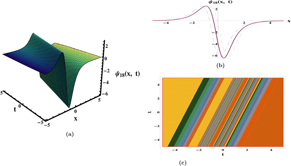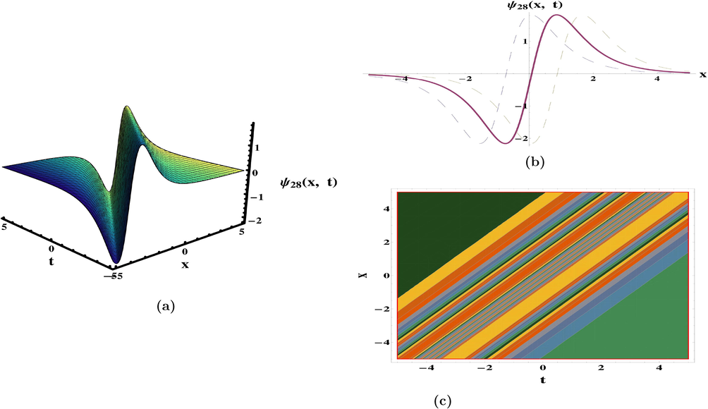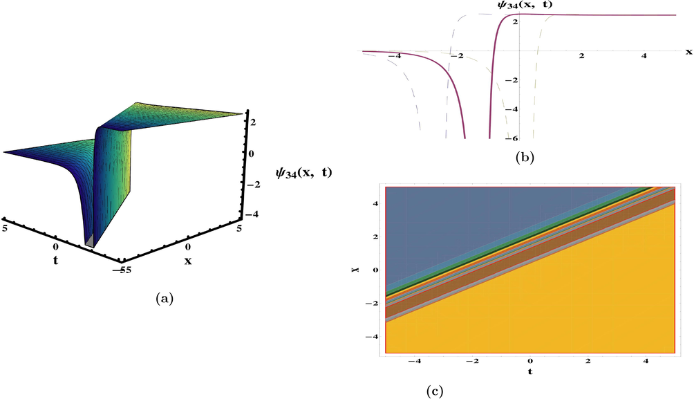In (Meng et al., 2011), periodic waves solutions have been recovered by integral bifurcation and semi-inverse approaches. The ansatz method to retrieve 1-soliton solution was also discussed. The categorization of bounded traveling wave solutions have been constructed in (da Silva, 2019). In diverse parameter regions, the dynamical deportment of traveling wave solutions and its bifurcations have been given in (Yu et al., 2016). The qualitative approach of planar systems to secure the bounded exact solutions were discussed (Zhong and Deng, 2017). The results obtained are exceptional and unique in comparison to previous findings in the literature. The periodic, kink, singular, anit-kink, combo kink-anti kink, and rational function (plane wave) solutions, which are appeared in Eqs. (47), (52), (56), (62), (64), (74) and (80) as exhibited in Figs. 1–7 respectively. The achievements reported in this article may be valuable in clarifying the true meaning of numerous nonlinear advancement circumstances that develop in various domains of nonlinear sciences.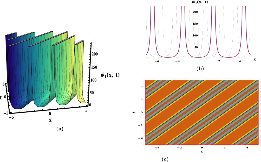

Plots of solution (47) for the parameters γ = - 1.5 , c = 0.8 , ν = 1.7 , λ = 0.7 , μ = 0.75 and B = e .

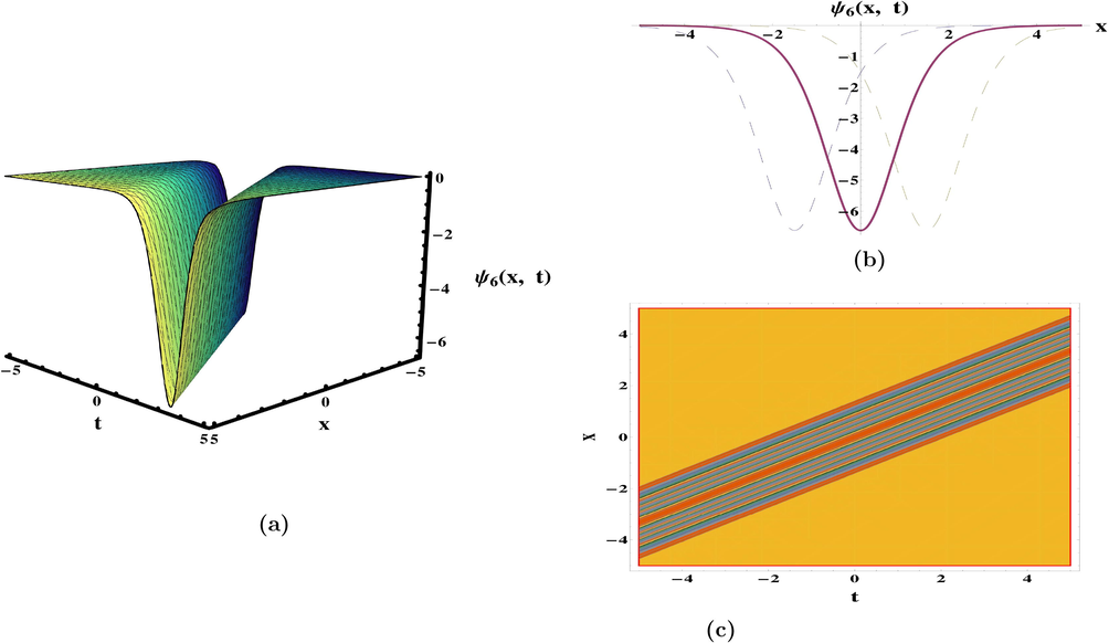
Plots of solution (52) for the parameters γ = - 2 , c = 1.5 , ν = 0.7 , λ = 1.1 , μ = - 0.7.5 and B = e .

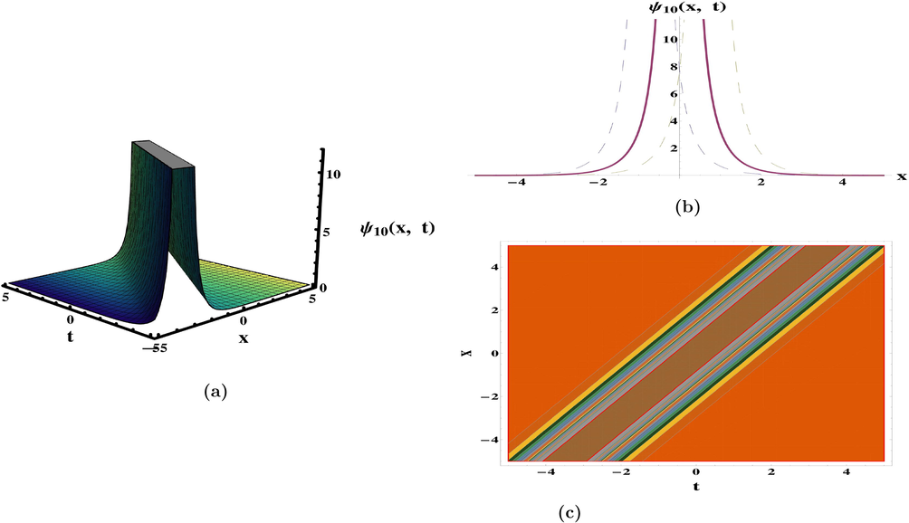
Plots of solution (56)for the parameters γ = - 1.1 , c = 0.7 , ν = 1.2 , λ = 0.75 , μ = - 0.65.5 and B = e .

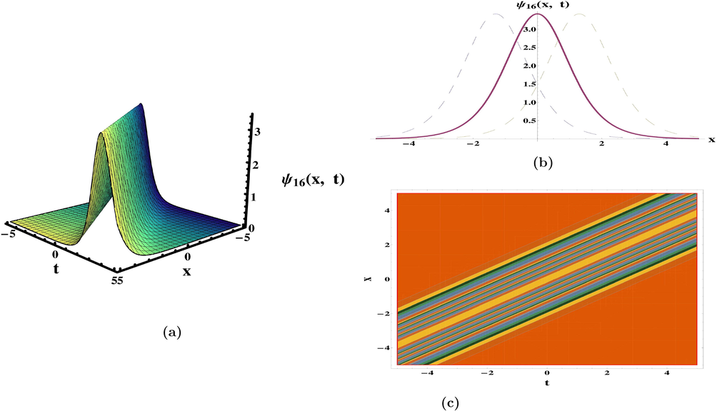
Plots of solution (62) for the parameters γ = 1.5 , c = 1.3 , ν = 0.6 , μ = - 0.9.5 and B = e .

Plots of solution (64) for the parameters p = 1.7 , q = 1.5 , γ = 1.4 , c = 0.3 , ν = 0.9 , λ = 0.7 , μ = - 0.5 and B = e .

Plots of solution (74) for the parameters p = 1.7 , q = 0.7 , γ = 1.5 , c = 0.8 , μ = 0.55 and B = e .

Plots of solution (80) for the parameters p = 0.7 , q = 1.7 , γ = 1.5 , c = 1.4 , r = 2 , λ = 2.4 , χ = 1.3 and B = e .

5 Concluding remarks

In this research work, we examined the new exact traveling wave structures to (1+1)-dimensional DGH system through mathematical technique known as NEDAM. By employing this mentioned norm we recovered several exact in the form of hyperbolic and trigonometric. The results obtained are exceptional and unique in comparison to previous findings in the literature. In addition, 3-dimensional, 2-dimensional, and corresponding contour graphs of earned outcomes are sketched in order to observe their dynamics with the choices of involved parameters. The outcomes retrieved in this article may be valuable in clarifying the true meaning of numerous nonlinear advancement circumstances that develop in various domains of applied sciences.

Acknowledgement

Taif University Researchers Supporting Project number (TURSP-2020/326), Taif University, Taif, Saudi Arabia.

Declaration of Competing Interest

The authors declare that they have no known competing financial interests or personal relationships that could have appeared to influence the work reported in this paper.

References

Marin M., Othman M.I.A., Seadawy A.R., Carstea C., . A domain of influence in the Moore-Gibson-Thompson theory of dipolar bodies. J. Taibah Univ. Sci.. 2020;14(1):653-660.
[Google Scholar]
Bhatti Muhammad M., Marin Marin, Zeeshan Ahmed, Ellahi R., Abdelsalam Sara I., . Swimming of motile gyrotactic microorganisms and nanoparticles in blood flow through anisotropically tapered arteries. Front. Phys.. 2020;8:1-12. Art. No. 95
[Google Scholar]
Khan Ambreen Afsar, Bukhari Syeda Rida, Marin Marin, Ellahi R., . Effects of chemical reaction on third-grade MHD fluid flow under the influence of heat and mass transfer with variable reactive index. Heat Transfer Res.. 2019;50(11):1061-1080.
[Google Scholar]
Seadawy A.R., Arshad M., Lu D., . Dispersive optical solitary wave solutions of strain wave equation in micro-structured solids and its applications. Physica A. 2020;540:123122
[Google Scholar]
Cao Yulei, Cheng Yi, He Jingsong, Chen Yiren, . High-order breather, M-kink lump and semi-rational solutions of Potential Kadomtsev-Petviashvili equation. Commun. Theor. Phys.. 2021;73(3)
[Google Scholar]
Yang Jiaopeng, Liu Rui, Chen Yiren, . Bifurcations of solitary waves of a simple equation. Int. J. Bifurcation Chaos. 2020;30(9):2050138.
[Google Scholar]
Chen Yiren, . New Generalized Soliton Solutions for a (3+1)-Dimensional Equation[J] Adv. Math. Phys.. 2020;2020
[Google Scholar]
Iqbal Mujahid, Seadawy Aly R., Dianchen Lu., . Construction of solitary wave solutions to the nonlinear modified Kortewege-de Vries dynamical equation in unmagnetized plasma via mathematical methods. Mod. Phys. Lett. A. 2018;33(32):1850183.
[Google Scholar]
Iqbal Mujahid, Seadawy Aly R., Khalil Omer H., Dianchen Lu., . Propagation of long internal waves in density stratified ocean for the (2+1)-dimensional nonlinear Nizhnik-Novikov-Vesselov dynamical equation. Results Phys.. 2020;16:102838
[Google Scholar]
Younis M., Sulaiman T.A., Bilal M., Rehman S.U., Younas U., . Modulation instability analysis, optical and other solutions to the modified nonlinear Schrödinger equation. Commu. Theor. Phys.. 2020;72:065001. (12pp)
[Google Scholar]
Rehman S.U., Ahmad J., . Modulation instability analysis and optical solitons in birefringent fibers to RKL equation without four wave mixing. Alexand. Eng. J.. 2020;60:1339-1354.
[Google Scholar]
Rezazadeh H., Korkmaz A., Eslami M., Mirhosseini-Alizamini S.M., . A large family of optical solutions to Kundu-Eckhaus model by a new auxiliary equation method. Opt. Quant. Electron.. 2019;51:84.
[Google Scholar]
Bilal M., Seadway A.R., Younis M., Rizvi S.T.R., Zahed H., . Dispersive of propagation wave solutions to unidirectional shallow water wave Dullin-Gottwald-Holm system and modulation instability analysis. Math. Meth. Appl. Sci. 2020 doi.10.1002/j.mma.7013
[Google Scholar]
Seadawy A.R., Lu D., Nasreen N., . Construction of solitary wave solutions of some nonlinear dynamical system arising in nonlinear water wave models. Indian J. Phys.. 2020;94:1785-1794.
[Google Scholar]
Syam M.I., . The solution of Cahn-Allen equation based on Bernoulli sub-equation method. Results Phys.. 2019;14:102413
[Google Scholar]
Abdou M.A., . On the fractional order space-time nonlinear equations arising in plasma physics. Indian J. Phys.. 2019;93:537-541.
[Google Scholar]
Younas U., Younis M., Seadawy A.R., Rizvi S.T.R., Althobaiti S., Sayed S., . Diverse exact solutions for modified nonlinear Schrödinger equation with conformable fractional derivative. Results Phys.. 2021;20:103766
[Google Scholar]
Rehman S.U., Seadawy A.R., Younis M., Rizvi S.T.R., Sulaiman T.A., Yusuf A., . Modulation instability analysis and optical solitons of the generalized model for description of propagation pulses in optical fiber with four non-linear terms. Modern Phys. Lett. B 2020
[CrossRef] [Google Scholar]
Olver Peter J., . Applications of Lie groups to differential equations. Springer-Verlag, New York, Inc; 2000.
Bluman George, Cheviakov Alexei, Anco Stephen, . Applications of Symmetry Methods to Partial Differential Equations. New York: Springer; 2009.
Seadawy Aly, Kumar Dipankar, Hosseini Kamyar, Samadani F., . The system of equations for the ion sound and Langmuir waves and its new exact solutions. Results Phys.. 2018;9:1631-1634.
[Google Scholar]
Çelik Nisa, Seadawy Aly R., Sağlam Özkan Yeşim, Yaşar Emrullah, . A model of solitary waves in a nonlinear elastic circular rod: Abundant different type exact solutions and conservation laws. Chaos Solitons Fractals. 2021;143:110486
[Google Scholar]
Khater A.H., Helal M.A., Seadawy A.R., . General soliton solutions of n-dimensional nonlinear Schrödinger equation. IL Nuovo Cimento. 2000;115B:1303-1312.
[Google Scholar]
Abd El-Hameed A.M., . Polydatin-loaded chitosan nanoparticles ameliorates early diabetic nephropathy by attenuating oxidative stress and inflammatory responses in streptozotocin-induced diabetic rat. J Diabetes Metab Disord. 2020;19:1599-1607.
[Google Scholar]
Seadawy Aly, . Two-dimensional interaction of a shear flow with a free surface in a stratified fluid and its a solitary wave solutions via mathematical methods. Eur. Phys. J. Plus. 2017;132:518.
[Google Scholar]
da Silva Priscila Leal, Freire Igor Leite, . Integrability, existence of global solutions, and wave breaking criteria for a generalization of the Camassa-Holm equation. Stud. Appl. Math.. 2020;145:537-562.
[Google Scholar]
Ancol Stephen C., da Silva Priscila Leal, Freire Igor Leite, . A family of wave-breaking equations generalizing the Camassa-Holm and Novikov equations. J. Math. Phys.. 2015;56:091506
[Google Scholar]
da Silva Priscila Leal, Freire Igor Leite, . Well-posedness, travelling waves and geometrical aspects of generalizations of the Camassa-Holm equation. J. Diff. Equ.. 2019;267:5318-5369.
[Google Scholar]
Younas U., Seadawy A.R., Younis M., Rizvi S.T.R., . Dispersive of propagation wave structures to the dullin-Gottwald-Holm dynamical equation in a shallow water waves. Chinese J. Phys.. 2020;68:348-364.
[Google Scholar]
Dullin H., Gottwald G., Holm D., . An integrable shallow water equation with linear and nonlinear dispersion. Phys. Rev. Lett.. 2001;87 Article 194501
[Google Scholar]
Mirhosseni-Alizamini S.M., Rezazadeh H., Srinivasa K., Bekir A., . New closed form solutions of the new coupled Konno-Oono equation using the new extended direct algebraic method. Pramana. 2020;94:52.
[Google Scholar]
Mustafa O.G., . Existence and uniqueness of low regularity solutions for the Dullin-Gottwald-Holm Equation. Commun. Math. Phys.. 2006;265:189-200.
[Google Scholar]
Zhou J., Tian L., Zhang W., . Sunil Kumar, Peakon-antipeakon interaction in the Dullin-Gottwald-Holm equation. Phys. Lett. A. 2013;377:1233-1238.
[Google Scholar]
Can X.G., Quang X.D., Qiang L.X., . Application of Exp-function method to Dullin-Gottwald-Holm equation. Appl. Math. Comput.. 2009;210:536-541.
[Google Scholar]
Tian L., Gui1 G., Liu Y., . On the well-posedness problem and the scattering problem for the Dullin-Gottwald-Holm Equation. Commun. Math. Phys.. 2005;257:667-701.
[Google Scholar]
Meng Q., He B., Long Y., Li Z., . New exact periodic wave solutions for the Dullin-Gottwald-Holm equation. Appl. Math. Comput.. 2011;218:4533-4537.
[Google Scholar]
da Silva P.L., . Classification of bounded travelling wave solutions for the Dullin-Gottwald-Holm equation. J. Math. Anal. Appl.. 2019;471:481-488.
[Google Scholar]
Yu W., . Exact solutions and bifurcations for the DGH equation. J. Appl. Anal. Comput.. 2016;6:968-980.
[Google Scholar]
Zhong J., Deng S., . Traveling Wave Solutions of a Two-Component Dullin-Gottwald-Holm System. J. Comput. Nonlinear Dyn.. 2017;12 031006-1
[Google Scholar]

Introduction

Analysis of NEDAM

Exact solutions

Results and discussion

Concluding remarks

Fulltext Views
26

PDF downloads
29

View/Download PDF
Download Citations

BibTeX
RIS

Show Sections

[1] Marin M., Othman M.I.A., Seadawy A.R., Carstea C., . A domain of influence in the Moore-Gibson-Thompson theory of dipolar bodies. J. Taibah Univ. Sci.. 2020;14(1):653-660.
[Google Scholar]

[2] Bhatti Muhammad M., Marin Marin, Zeeshan Ahmed, Ellahi R., Abdelsalam Sara I., . Swimming of motile gyrotactic microorganisms and nanoparticles in blood flow through anisotropically tapered arteries. Front. Phys.. 2020;8:1-12. Art. No. 95
[Google Scholar]

[3] Khan Ambreen Afsar, Bukhari Syeda Rida, Marin Marin, Ellahi R., . Effects of chemical reaction on third-grade MHD fluid flow under the influence of heat and mass transfer with variable reactive index. Heat Transfer Res.. 2019;50(11):1061-1080.
[Google Scholar]

[4] Seadawy A.R., Arshad M., Lu D., . Dispersive optical solitary wave solutions of strain wave equation in micro-structured solids and its applications. Physica A. 2020;540:123122
[Google Scholar]

[5] Cao Yulei, Cheng Yi, He Jingsong, Chen Yiren, . High-order breather, M-kink lump and semi-rational solutions of Potential Kadomtsev-Petviashvili equation. Commun. Theor. Phys.. 2021;73(3)
[Google Scholar]

[6] Yang Jiaopeng, Liu Rui, Chen Yiren, . Bifurcations of solitary waves of a simple equation. Int. J. Bifurcation Chaos. 2020;30(9):2050138.
[Google Scholar]

[7] Chen Yiren, . New Generalized Soliton Solutions for a (3+1)-Dimensional Equation[J] Adv. Math. Phys.. 2020;2020
[Google Scholar]

[8] Iqbal Mujahid, Seadawy Aly R., Dianchen Lu., . Construction of solitary wave solutions to the nonlinear modified Kortewege-de Vries dynamical equation in unmagnetized plasma via mathematical methods. Mod. Phys. Lett. A. 2018;33(32):1850183.
[Google Scholar]

[9] Iqbal Mujahid, Seadawy Aly R., Khalil Omer H., Dianchen Lu., . Propagation of long internal waves in density stratified ocean for the (2+1)-dimensional nonlinear Nizhnik-Novikov-Vesselov dynamical equation. Results Phys.. 2020;16:102838
[Google Scholar]

[10] Younis M., Sulaiman T.A., Bilal M., Rehman S.U., Younas U., . Modulation instability analysis, optical and other solutions to the modified nonlinear Schrödinger equation. Commu. Theor. Phys.. 2020;72:065001. (12pp)
[Google Scholar]

[11] Rehman S.U., Ahmad J., . Modulation instability analysis and optical solitons in birefringent fibers to RKL equation without four wave mixing. Alexand. Eng. J.. 2020;60:1339-1354.
[Google Scholar]

[12] Rezazadeh H., Korkmaz A., Eslami M., Mirhosseini-Alizamini S.M., . A large family of optical solutions to Kundu-Eckhaus model by a new auxiliary equation method. Opt. Quant. Electron.. 2019;51:84.
[Google Scholar]

[13] Bilal M., Seadway A.R., Younis M., Rizvi S.T.R., Zahed H., . Dispersive of propagation wave solutions to unidirectional shallow water wave Dullin-Gottwald-Holm system and modulation instability analysis. Math. Meth. Appl. Sci. 2020 doi.10.1002/j.mma.7013
[Google Scholar]

[14] Seadawy A.R., Lu D., Nasreen N., . Construction of solitary wave solutions of some nonlinear dynamical system arising in nonlinear water wave models. Indian J. Phys.. 2020;94:1785-1794.
[Google Scholar]

[15] Syam M.I., . The solution of Cahn-Allen equation based on Bernoulli sub-equation method. Results Phys.. 2019;14:102413
[Google Scholar]

[16] Abdou M.A., . On the fractional order space-time nonlinear equations arising in plasma physics. Indian J. Phys.. 2019;93:537-541.
[Google Scholar]

[17] Younas U., Younis M., Seadawy A.R., Rizvi S.T.R., Althobaiti S., Sayed S., . Diverse exact solutions for modified nonlinear Schrödinger equation with conformable fractional derivative. Results Phys.. 2021;20:103766
[Google Scholar]

[18] Rehman S.U., Seadawy A.R., Younis M., Rizvi S.T.R., Sulaiman T.A., Yusuf A., . Modulation instability analysis and optical solitons of the generalized model for description of propagation pulses in optical fiber with four non-linear terms. Modern Phys. Lett. B 2020
[CrossRef] [Google Scholar]

[19] Olver Peter J., . Applications of Lie groups to differential equations. Springer-Verlag, New York, Inc; 2000.

[20] Bluman George, Cheviakov Alexei, Anco Stephen, . Applications of Symmetry Methods to Partial Differential Equations. New York: Springer; 2009.

[21] Seadawy Aly, Kumar Dipankar, Hosseini Kamyar, Samadani F., . The system of equations for the ion sound and Langmuir waves and its new exact solutions. Results Phys.. 2018;9:1631-1634.
[Google Scholar]

[22] Çelik Nisa, Seadawy Aly R., Sağlam Özkan Yeşim, Yaşar Emrullah, . A model of solitary waves in a nonlinear elastic circular rod: Abundant different type exact solutions and conservation laws. Chaos Solitons Fractals. 2021;143:110486
[Google Scholar]

[23] Khater A.H., Helal M.A., Seadawy A.R., . General soliton solutions of n-dimensional nonlinear Schrödinger equation. IL Nuovo Cimento. 2000;115B:1303-1312.
[Google Scholar]

[24] Abd El-Hameed A.M., . Polydatin-loaded chitosan nanoparticles ameliorates early diabetic nephropathy by attenuating oxidative stress and inflammatory responses in streptozotocin-induced diabetic rat. J Diabetes Metab Disord. 2020;19:1599-1607.
[Google Scholar]

[25] Seadawy Aly, . Two-dimensional interaction of a shear flow with a free surface in a stratified fluid and its a solitary wave solutions via mathematical methods. Eur. Phys. J. Plus. 2017;132:518.
[Google Scholar]

[26] da Silva Priscila Leal, Freire Igor Leite, . Integrability, existence of global solutions, and wave breaking criteria for a generalization of the Camassa-Holm equation. Stud. Appl. Math.. 2020;145:537-562.
[Google Scholar]

[27] Ancol Stephen C., da Silva Priscila Leal, Freire Igor Leite, . A family of wave-breaking equations generalizing the Camassa-Holm and Novikov equations. J. Math. Phys.. 2015;56:091506
[Google Scholar]

[28] da Silva Priscila Leal, Freire Igor Leite, . Well-posedness, travelling waves and geometrical aspects of generalizations of the Camassa-Holm equation. J. Diff. Equ.. 2019;267:5318-5369.
[Google Scholar]

[29] Younas U., Seadawy A.R., Younis M., Rizvi S.T.R., . Dispersive of propagation wave structures to the dullin-Gottwald-Holm dynamical equation in a shallow water waves. Chinese J. Phys.. 2020;68:348-364.
[Google Scholar]

[30] Dullin H., Gottwald G., Holm D., . An integrable shallow water equation with linear and nonlinear dispersion. Phys. Rev. Lett.. 2001;87 Article 194501
[Google Scholar]

[31] Mirhosseni-Alizamini S.M., Rezazadeh H., Srinivasa K., Bekir A., . New closed form solutions of the new coupled Konno-Oono equation using the new extended direct algebraic method. Pramana. 2020;94:52.
[Google Scholar]

[32] Mustafa O.G., . Existence and uniqueness of low regularity solutions for the Dullin-Gottwald-Holm Equation. Commun. Math. Phys.. 2006;265:189-200.
[Google Scholar]

[33] Zhou J., Tian L., Zhang W., . Sunil Kumar, Peakon-antipeakon interaction in the Dullin-Gottwald-Holm equation. Phys. Lett. A. 2013;377:1233-1238.
[Google Scholar]

[34] Can X.G., Quang X.D., Qiang L.X., . Application of Exp-function method to Dullin-Gottwald-Holm equation. Appl. Math. Comput.. 2009;210:536-541.
[Google Scholar]

[35] Tian L., Gui1 G., Liu Y., . On the well-posedness problem and the scattering problem for the Dullin-Gottwald-Holm Equation. Commun. Math. Phys.. 2005;257:667-701.
[Google Scholar]

[36] Meng Q., He B., Long Y., Li Z., . New exact periodic wave solutions for the Dullin-Gottwald-Holm equation. Appl. Math. Comput.. 2011;218:4533-4537.
[Google Scholar]

[37] da Silva P.L., . Classification of bounded travelling wave solutions for the Dullin-Gottwald-Holm equation. J. Math. Anal. Appl.. 2019;471:481-488.
[Google Scholar]

[38] Yu W., . Exact solutions and bifurcations for the DGH equation. J. Appl. Anal. Comput.. 2016;6:968-980.
[Google Scholar]

[39] Zhong J., Deng S., . Traveling Wave Solutions of a Two-Component Dullin-Gottwald-Holm System. J. Comput. Nonlinear Dyn.. 2017;12 031006-1
[Google Scholar]

Dynamical behaviour of shallow water waves and solitary wave solutions of the Dullin-Gottwald-Holm dynamical system

Abstract

Keywords

Shallow water waves

Solitary water waves

(1+1)-Dimensional DGH system

NEDAM

Integrability

1 Introduction

2 Analysis of NEDAM

3 Exact solutions

4 Results and discussion

5 Concluding remarks

Acknowledgement

Declaration of Competing Interest

References

Suggested read for related articles: