

Translate this page into:
Estimation methods for the discrete Poisson-Lindley and discrete Lindley distributions with actuarial measures and applications in medicine
⁎Corresponding author. ahmed.afify@fcom.bu.edu.eg (Ahmed Z. Afify)
-
Received: ,
Accepted: ,
This article was originally published by Elsevier and was migrated to Scientific Scholar after the change of Publisher.
Peer review under responsibility of King Saud University.
Abstract
Discrete distributions have their important in modeling count data in several applied fields such as epidemiology, public health, sociology, medicine, and agriculture. This paper discusses the estimation of the parameters of two discrete models called discrete Poisson-Lindley and discrete Lindley distributions, using several frequentist estimation methods. Parameter estimation can provide a guideline for choosing the best method of estimation for the model parameters, which would be very important to reliability engineers and applied statisticians. The finite sample properties of the estimates are explored using extensive simulation results. The ordering performance of the proposed estimators is determined by the partial and overall ranks of different parametric values. We also derived two important actuarial measures of the two discrete models. A computational study for the two risk measures is conducted. Finally, applications of the two discrete distributions have been examined and compared with other discrete distributions via three data sets from the medicine field including two COVID-19 data sets.
Keywords
Bootstrap confidence intervals
COVID-19 data
Discrete-Lindley distribution
Discrete Poisson-Lindley distribution
Percentile estimation
TVaR

1 Introduction
The discrete distributions are very useful in modeling count data in several applied fields such as medicine, public health, epidemiology, agriculture, sociology, and applied science. Many discrete distributions have been proposed for modeling count data. However, the traditional discrete distributions including geometric and Poisson have limited applicability as models for failure times, reliability, counts, etc. This is so, since many real count data show either under-dispersion, in which the variance is smaller than the mean or over-dispersion, in which the variance is greater than the mean. This has motivated many authors to develop some new discrete distributions based on classical continuous distributions for failure times, reliability, etc.
Sankaran (1970) introduced the discrete Poisson-Lindley (DPL) distribution which is specified by the probability mass function (PMF)
Bakouch et al. (2014) proposed the discrete Lindley (DL) distribution as a discrete version of the continuous Lindley distribution. The PMF of the DL distribution takes the form
Our aim in this paper is to explore the estimation of the DPL and DL parameters by five methods of estimation, such as the maximum likelihood estimator (MLE), Cramér-von Mises estimator (CVME), least-square estimator (OLSE), weighted least squares estimator (WLSE) and percentile estimator (PCE). We compare the proposed estimators using an extensive computational simulations to develop a guideline for choosing the best estimation method that provides better estimates for the parameters of the DPL and DL models.
In this regard, comparing several frequentist estimators for estimating the parameters of different continuous distributions are conducted by several authors. Notable among them are Dey et al. (2017), Nassar et al. (2018), Rodrigues et al. (2018), Afify and Mohamed (2020), Shakhatreh et al. (2020), Afify et al. (2020), Al-Mofleh et al. (2020), Aldahlan and Afify (2020) and Nassar et al. (2020) for exponentiated-Gumbel, transmuted exponentiated Pareto, Poisson-exponential, extended odd Weibull exponential, generalized extended exponential Weibull, generalized Ramos-Louzada, exponentiated half-logistic exponential and alpha power-exponential distributions.
As far as we know, there are no reports on estimation of parameters of the DPL and DL distribution based on several frequentist estimators. To the best of our knowledge, Sankaran (1970) proposed the moments and maximum likelihood methods for estimating the DPL parameter. However, he only used the moments estimator for the two analyzed data sets he studied. Ghitany and Al-Mutairi (2009) presented a simulation study to compare the moments and maximum likelihood estimators and showed that the two estimators are consistent and asymptotically normal.
Further, we derive two important risk measures for the DPL and DL distributions, called value at risk and tail value at risk which are useful in evaluating the exposure to market risk in a portfolio of instruments. The numerical simulations of the two risk measures are presented for the two discrete distributions using several parametric values.
The rest of the paper is organized as follows. In Section 2, we derive the value at risk and tail value at risk for the DPL and DL distributions along with detailed numerical simulations for these measures. In Section 3, different classical methods of parameter estimation are discussed. In Section 4, we present the simulation results to compare and assess the performance of the proposed estimators. Three COVID-19 data sets are analyzed to validate the use of DPL and DL distributions in fitting lifetime count data are explored in Section 5. Finally, concluding remarks are presented in Section 6.
2 Actuarial measures
In this section, we determine the value at risk (VaR) and tail value at risk (TVaR) for the DPL and DL distributions, which play a crucial role in portfolio optimization under uncertainty.
2.1 VaR measure
The VaR of any random variable X is the quantile of its CDF as shown in Artzner (1999), and it is defined, for a probability level , by .
The VaR of the DPL distribution with PMF (1) is derived as The VaR of the DL model with PMF (5) takes the form
2.2 TVaR Measure
The TVaR is an important actuarial measure, and it is used to determine the expected value of the loss given that an event outside a given probability level has occurred. The TVaR is defined in Klugman et al. (2012) by the following equation Using Eqs. (3) and (4), the TVaR of the DPL distribution is derived as Similarly, based on Eqs. (7) and (8), the TVaR of the DL distribution follows as
2.3 Simulations for risk measures
In this sub-section, we present some numerical computations for the VaR and TVaR measures of the DPL and DL distributions for different parametric values. The results can be obtained as follows.
-
A random sample of size is generated from the DPL and DL distributions and their parameters are estimated by the maximum likelihood method.
-
The VaR and TVaR of the two distributions are calculated from 2,000 repetitions.
| Significance Level | DPL( ) | DL( ) |
|---|---|---|
| 0.70 | 8.90197 | 8.26617 |
| 0.75 | 9.95805 | 9.2078 |
| 0.80 | 11.21761 | 10.32968 |
| 0.85 | 12.79907 | 11.73696 |
| 0.90 | 14.96585 | 13.66341 |
| 0.95 | 18.5491 | 16.84654 |
| 0.99 | 26.50909 | 23.91149 |
| Significance Level | DPL( ) | DL( ) |
| 0.70 | 4.03788 | 3.50114 |
| 0.75 | 4.56447 | 3.9304 |
| 0.80 | 5.19558 | 4.44301 |
| 0.85 | 5.99151 | 5.08736 |
| 0.90 | 7.08663 | 5.97111 |
| 0.95 | 8.90529 | 7.43411 |
| 0.99 | 12.96347 | 10.68758 |
| Significance Level | DPL( ) | DL( ) |
| 0.70 | 1.02010 | 0.51384 |
| 0.75 | 1.17239 | 0.58836 |
| 0.80 | 1.35813 | 0.67874 |
| 0.85 | 1.59661 | 0.79409 |
| 0.90 | 1.93101 | 0.95472 |
| 0.95 | 2.49861 | 1.22504 |
| 0.99 | 3.8006 | 1.83774 |
| Significance Level | DPL( ) | DL( ) |
|---|---|---|
| 0.70 | 13.81718 | 12.58693 |
| 0.75 | 14.79489 | 13.45659 |
| 0.80 | 15.97354 | 14.50447 |
| 0.85 | 17.46878 | 15.83318 |
| 0.90 | 19.53854 | 17.67156 |
| 0.95 | 22.99892 | 20.74363 |
| 0.99 | 30.78289 | 27.65028 |
| Significance Level | DPL( ) | DL( ) |
| 0.70 | 6.28894 | 5.23761 |
| 0.75 | 6.78275 | 5.63693 |
| 0.80 | 7.37937 | 6.11848 |
| 0.85 | 8.13786 | 6.72957 |
| 0.90 | 9.19001 | 7.57572 |
| 0.95 | 10.9531 | 8.99085 |
| 0.99 | 14.92949 | 12.17532 |
| Significance Level | DPL( ) | DL( ) |
| 0.70 | 1.44267 | 0.59833 |
| 0.75 | 1.59315 | 0.67166 |
| 0.80 | 1.7768 | 0.76072 |
| 0.85 | 2.01277 | 0.87453 |
| 0.90 | 2.34394 | 1.03330 |
| 0.95 | 2.90669 | 1.30100 |
| 0.99 | 4.1999 | 1.90943 |
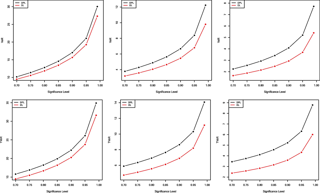
- Plots of the VaR (top panel) and TVaR (bottom panel) of the DPL and DL distributions using the values in Tables 1 and 2.
The results in Tables 1 and 2 and the plots in Fig. 1 reveal that the VaR and TVaR measures are increasing functions in the parameter , for the DPL distribution, and , for the DL distribution.
3 Estimation methods
In this section, we discuss the estimation of the parameters of the DPL and DL distributions using several classical methods of estimation including the maximum likelihood estimator (MLE), Cramér-von Mises estimator (CVE), least-squares estimator (LSE), weighted least squares estimator (WLSE) and percentile estimator (PCE).
3.1 Maximum likelihood estimation
Let
be a random sample of size n from the DPL model with PMF (2), then the log-likelihood function reduces to
Let
be a random sample of size n from the DL model with PMF (5), then the log-likelihood function is given by
3.2 Least-squares and weighted least-squares estimation
Let
be the order statistics from the DPL distribution. By minimizing the following equation, we have LSE (Swain et al., 1988) of the parameter
of the DPL distribution
it can be also obtained by solving the following non-linear equation
where
Let
be the order statistics of a random sample from the DL distribution. The LSE of the DL parameter
follows by minimizing the following equation with respect to
The LSE of
can also be obtained by solving the following non-linear equation
where
3.3 Cramér-von Mises Estimation
The CVME of the parameter of the DPL distribution is obtained by minimizing the following equation or by solving the following non-linear equation where is defined in Eq. (13). Further details about the CVME can be explored in Macdonald (1971) and Luceño (2006). The CVME of the DL parameter can be calculated by minimizing the following equation or by solving the following non-linear equation where is given in Eq. (14).
3.4 Percentile Estimation
This estimation method was introduced by Kao (1958, 1959). Let be an estimate of , then the PCE of DPL parameter follows by minimizing where We can also obtain the PCE of the parameter by solving the following non-linear equation where Let is an estimate of , then the PCE of the DL parameter follows by minimizing The PCE of the parameter can also be determined by solving the non-linear equation where
4 Simulation Study
In this section, the performance of different estimation methods for estimating the DPL( ) and DL( ) parameters is explored via numerical simulations. Different sample sizes, , and several parametric values are considered for the parameters and . We generate random samples from the two distributions using Eqs. (3) and (7), respectively. The performance of these estimators are assessed by determining some indices such as the average values of the estimates (AVEs), average mean square errors (MSEs), average absolute biases (ABBs), and average mean relative estimates (MREs) for all sample sizes and parametric combinations using the R software©.
These indices can be determined using the following equations where or .
Simulation results including AVEs, ABBs, MSEs and MREs for the two parameters
and
of the DPL and DL distributions using several estimation approaches are reported in Tables 3–6. Additionally, these tables illustrate the rank of each estimator among all the five estimators which is represented by superscript indicators in each row and the
which is represented by the partial sum of ranks in each column for every sample size.
n
Est.
MLE
CVME
LSE
PCE
WLSE
20
AVEs
0.19606
0.20512
0.20529
0.19537
0.20363
ABBs
MSEs
MREs
Ranks
40
AVEs
0.19276
0.20266
0.20228
0.19585
0.20133
ABBs
MSEs
MREs
Ranks
60
AVEs
0.19162
0.20134
0.20073
0.19573
0.20103
ABBs
MSEs
MREs
Ranks
80
AVEs
0.19137
0.20129
0.20019
0.19652
0.20056
ABBs
MSEs
MREs
Ranks
100
AVEs
0.19106
0.20086
0.20045
0.19704
0.20071
ABBs
MSEs
MREs
Ranks
20
AVEs
0.45460
0.51588
0.50524
0.48614
0.50106
ABBs
MSEs
MREs
Ranks
40
AVEs
0.44802
0.50510
0.50127
0.48845
0.50064
ABBs
MSEs
MREs
Ranks
60
AVEs
0.44914
0.49937
0.49984
0.48864
0.49723
ABBs
MSEs
MREs
Ranks
80
AVEs
0.44615
0.50067
0.50012
0.48867
0.49659
ABBs
MSEs
MREs
Ranks
100
AVEs
0.44547
0.49984
0.49761
0.49103
0.49653
ABBs
MSEs
MREs
Ranks
n
Est.
MLE
CVME
LSE
PCE
WLSE
20
AVEs
0.82634
1.00301
0.98853
0.39414
0.98526
ABBs
MSEs
MREs
Ranks
40
AVEs
0.81185
0.98221
0.97546
0.39857
0.97555
ABBs
MSEs
MREs
Ranks
60
AVEs
0.80381
0.97510
0.97837
0.40102
0.97408
ABBs
MSEs
MREs
Ranks
80
AVEs
0.80129
0.96981
0.97179
0.40182
0.97040
ABBs
MSEs
MREs
Ranks
100
AVEs
0.80080
0.97775
0.96876
0.40777
0.97156
ABBs
MSEs
MREs
Ranks
20
AVEs
1.13242
1.45882
1.42722
1.47038
1.43834
ABBs
MSEs
MREs
Ranks
40
AVEs
1.10559
1.41598
1.40194
1.47368
1.43224
ABBs
MSEs
MREs
Ranks
60
AVEs
1.09942
1.40902
1.40520
1.46148
1.43142
ABBs
MSEs
MREs
Ranks
80
AVEs
1.09837
1.40565
1.40449
1.46497
1.41964
ABBs
MSEs
MREs
Ranks
100
AVEs
1.09223
1.39648
1.39322
1.47211
1.42241
ABBs
MSEs
MREs
Ranks
n
Est.
MLE
CVME
LSE
PCE
WLSE
20
AVEs
0.20428
0.21867
0.21764
0.19561
0.21647
ABBs
0.02624{1}
0.03455{4}
0.03515{5}
0.02759{2}
0.03290{3}
MSEs
0.00113{1}
0.45543{5}
0.00224{3}
0.00117{2}
0.00662{4}
MREs
0.13122{1}
0.17276{4}
0.17576{5}
0.13794{3}
0.16450{2}
Ranks
40
AVEs
0.20179
0.21546
0.21517
0.19499
0.21510
ABBs
0.01819{1}
0.02512{5}
0.02509{4}
0.01912{2}
0.02470{3}
MSEs
0.00054{1}
0.44796{5}
0.00111{3}
0.00057{2}
0.00489{4}
MREs
0.09097{1}
0.12561{5}
0.12543{4}
0.09560{2}
0.12348{3}
Ranks
60
AVEs
0.20131
0.21501
0.21413
0.19588
0.21386
ABBs
0.01507{1}
0.02128{4}
0.02150{5}
0.01566{2}
0.02058{3}
MSEs
0.00036{1}
0.44746{5}
0.00076{3}
0.00037{2}
0.00416{4}
MREs
0.07537{1}
0.10641{4}
0.10748{5}
0.07832{2}
0.10290{3}
Ranks
80
AVEs
0.20195
0.21412
0.21352
0.19634
1.41964
ABBs
0.01258{1}
0.01948{4}
0.01927{3}
0.01344{2}
0.21311{5}
MSEs
0.00026{1}
0.44678{5}
0.00060{3}
0.00028{2}
0.01814{4}
MREs
0.06291{2}
0.09740{5}
0.09633{4}
0.06718{3}
0.00393{1}
Ranks
100
AVEs
0.20061
0.21319
0.21407
0.19668
0.21336
ABBs
0.01161{1}
0.01757{4}
0.01809{5}
0.01189{2}
0.01713{3}
MSEs
0.00021{1}
0.44578{5}
0.00051{3}
0.00023{2}
0.00376{4}
MREs
0.05804{1}
0.08784{4}
0.09044{5}
0.05943{2}
0.08563{3}
Ranks
20
AVEs
0.45543
0.50757
0.50711
0.48569
0.50300
ABBs
0.06791{2}
0.07239{4}
0.07257{5}
0.06734{1}
0.06946{3}
MSEs
0.00662{1}
0.00900{5}
0.00897{4}
0.00723{2}
0.00795{3}
MREs
0.13582{2}
0.14478{4}
0.14514{5}
0.13468{1}
0.13892{3}
Ranks
40
AVEs
0.44796
0.50448
0.50012
0.48775
0.49911
ABBs
0.05983{5}
0.05015{4}
0.05004{3}
0.04821{1}
0.04852{2}
MSEs
0.00489{5}
0.00414{4}
0.00397{3}
0.00360{1}
0.00371{2}
MREs
0.11966{5}
0.10030{4}
0.10008{3}
0.09643{1}
0.09704{2}
Ranks
60
AVEs
0.44746
0.49718
0.50018
0.48812
0.49580
ABBs
0.05631{5}
0.03982{2}
0.04011{3}
0.04035{4}
0.03790{1}
MSEs
0.00416{5}
0.00250{2}
0.00257{4}
0.00253{3}
0.00227{1}
MREs
0.11263{5}
0.07963{2}
0.08021{3}
0.08069{4}
0.07580{1}
Ranks
80
AVEs
0.44678
0.49888
0.49745
0.49242
0.49762
ABBs
0.05524{5}
0.03556{3}
0.03569{4}
0.03517{2}
0.03347{1}
MSEs
0.00393{5}
0.00196{3}
0.00200{4}
0.00191{2}
0.00176{1}
MREs
0.11048{5}
0.07111{3}
0.07138{4}
0.07035{2}
0.06694{1}
Ranks
100
AVEs
0.44578
0.49805
0.49762
0.49246
0.49460
ABBs
0.05516{5}
0.03122{2}
0.03192{4}
0.03160{3}
0.02976{1}
MSEs
0.00376{5}
0.00153{2}
0.00161{4}
0.00154{3}
0.00141{1}
MREs
0.11033{5}
0.06245{2}
0.06385{4}
0.06319{3}
0.05952{1}
Ranks
n
Est.
MLE
CVME
LSE
PCE
WLSE
20
AVEs
0.82182
0.97809
0.96423
0.38079
0.97326
ABBs
0.19066{5}
0.13673{2}
0.13624{1}
0.14081{4}
0.13880{3}
MSEs
0.04606{4}
1.12290{5}
0.02838{1}
0.03222{3}
0.03047{2}
MREs
0.19066{5}
0.13673{2}
0.13624{1}
0.14081{4}
0.13880{3}
Ranks
40
AVEs
0.80929
0.96822
0.96475
0.38904
0.96779
ABBs
0.19194{5}
0.09707{1}
0.09854{2}
0.10242{3}
0.10261{4}
MSEs
0.04282{4}
1.11120{5}
0.01488{1}
0.01615{3}
0.01603{2}
MREs
0.19194{5}
0.09707{1}
0.09854{2}
0.10242{3}
0.10261{4}
Ranks
60
AVEs
0.80397
0.96037
0.96231
0.39034
0.96423
ABBs
0.19624{5}
0.08432{4}
0.08163{1}
0.08230{2}
0.08331{3}
MSEs
0.04263{4}
1.10966{5}
0.01014{1}
0.01056{2}
0.01059{3}
MREs
0.19624{5}
0.08432{4}
0.08163{1}
0.08230{2}
0.08331{3}
Ranks
80
AVEs
0.80331
0.96340
0.95640
0.39368
0.96558
ABBs
0.19673{5}
0.07436{3}
0.07544{4}
0.07339{2}
0.07205{1}
MSEs
0.04193{4}
1.10632{5}
0.00847{3}
0.00828{2}
0.00789{1}
MREs
0.19673{5}
0.07436{3}
0.07544{4}
0.07339{2}
0.07205{1}
Ranks
100
AVEs
0.80240
0.96210
0.95805
0.39654
0.96737
ABBs
0.19760{5}
0.06718{3}
0.06812{4}
0.06577{1}
0.06624{2}
MSEs
0.04160{4}
1.10346{5}
0.00699{3}
0.00664{2}
0.00663{1}
MREs
0.19760{5}
0.06718{3}
0.06812{4}
0.06577{1}
0.06624{2}
Ranks
20
AVEs
1.12290
1.38100
1.36864
1.46240
1.40862
ABBs
0.38079{5}
0.21436{3}
0.21037{1}
0.23352{4}
0.21259{2}
MSEs
0.16817{5}
0.06645{2}
0.06416{1}
0.08795{4}
0.06797{3}
MREs
0.25386{5}
0.14290{3}
0.14025{1}
0.15568{4}
0.14173{2}
Ranks
40
AVEs
1.11120
1.36654
1.36327
1.46978
1.41346
ABBs
0.38904{5}
0.17306{3}
0.17496{4}
0.16748{2}
0.16515{1}
MSEs
0.16322{5}
0.04279{3}
0.04275{2}
0.04293{4}
0.04105{1}
MREs
0.25936{5}
0.11537{3}
0.11664{4}
0.11165{2}
0.11010{1}
Ranks
60
AVEs
1.10966
1.36881
1.36059
1.47028
1.41498
ABBs
0.39034{5}
0.15704{3}
0.15872{4}
0.13801{1}
0.14123{2}
MSEs
0.16099{5}
0.03448{3}
0.03479{4}
0.02881{1}
0.02943{2}
MREs
0.26023{5}
0.10469{3}
0.10581{4}
0.09201{1}
0.09415{2}
Ranks
80
AVEs
1.10632
1.36635
1.36064
1.47588
1.41368
ABBs
0.39368{5}
0.14766{3}
0.15346{4}
0.11639{1}
0.12443{2}
MSEs
0.16079{5}
0.02978{3}
0.03201{4}
0.02114{1}
0.02258{2}
MREs
0.26245{5}
0.09844{3}
0.10231{4}
0.07759{1}
0.08295{2}
Ranks
100
AVEs
1.10346
1.36260
1.36113
1.47760
1.41373
ABBs
0.39654{5}
0.14799{4}
0.14687{3}
0.10493{1}
0.11783{2}
MSEs
0.16058{5}
0.02903{4}
0.02836{3}
0.01690{1}
0.02007{2}
MREs
0.26436{5}
0.09866{4}
0.09791{3}
0.06996{1}
0.07856{2}
Ranks
One can note that the parameter estimates for both distributions are entirely good, that is, these estimates are quite reliable and very close to the true parameter values, showing small ABBs, MSEs and MREs for all values of the parameters and . The five estimators achieve the consistency property, where the MSEs, ABBs and MREs decrease as n increases, for all considered parametric values.
The performance ordering of these estimators is determined based on the partial and overall rank of the introduced estimators for both DPL and DL distributions which are listed in Table 7. Based on Table 7, we conclude that the performance ordering of these estimators, for the DPL distribution, from best to worst is WLSE, LSE, PCE, CVME, and MLE for all the studied cases. Furthermore, the performance ordering of these estimators, for the DL model, from best to worst is PCE, WLSE, LSE, CVME, and MLE for all the studied cases.
DPL
Parameter
n
MLE
CVME
LSE
PCE
WLSE
20
1
4
5
3
2
40
1
5
4
2
3
60
1
5
4
3
2
80
2
5
3
4
1
100
5
3
4
1
2
20
1
5
4
3
2
40
4.5
4.5
2
3
1
60
5
2
3
4
1
80
5
3
4
2
1
100
5
2
4
3
1
20
4
4
1.5
4
1.5
40
4.5
4.5
1
2.5
2.5
60
3.5
3.5
2
5
1
80
5
1
4
2.5
2.5
100
5
4
1
3
2
20
4.5
3
1
4.5
2
40
5
2
1
4
3
60
5
2
1
4
3
80
5
4
2.5
2.5
1
100
5
4
3
1.5
1.5
Ranks
77
70.5
55
61.5
36
Overall Rank
5
4
2
3
1
DL
Parameter
n
MLE
CVME
LSE
PCE
WLSE
20
1
4.5
4.5
2
3
40
1
5
4
2
3
60
1
4.5
4.5
2
3
80
1
5
3.5
2
3.5
100
1
4.5
4.5
2
3
20
2
4
5
1
3
40
5
4
3
1
2
60
5
2
3
4
1
80
5
3
4
2
1
100
5
2
4
3
1
20
5
3
1
4
2
40
5
2
1
3
4
60
5
4
1
2
3
80
5
3.5
3.5
2
1
100
5
3.5
3.5
1
2
20
5
3
1
4
2
40
5
3
4
2
1
60
5
3
4
1
2
80
5
3
4
1
2
100
5
4
3
1
2
Ranks
77
70.5
66
42
44.5
Overall Rank
5
4
3
1
2
In summary, we can conclude that the weighted least-squares method outperforms all other considered estimation methods with overall score of 36, hence this method is recommended to estimate the parameter of the DPL distribution, whereas the percentile method is recommended to estimate the DL parameter due to its superiority with overall rank of 42.
5 Modeling medicine data
In this section, we use three real-life data sets from medical science to show the superiority of the DPL and DL distributions by comparing them with some well-known discrete distributions such as discrete Pareto (DP) (Krishna and Pundir, 2009), discrete Burr (DB) (Krishna and Pundir, 2009) and discrete Burr-Hatke (DBH) (El-Morshedy et al., 2020) distributions.
The first data set contains 20 observations about the numbers of daily deaths in Saudi Arabia due to COVID-19 infections from 24 March to 12 April, 2020. The second data set contains 20 observations about the numbers of daily recover patients in Saudi Arabia from COVID-19 infections from 24 March to 12 April, 2020. The first and second data sets are reported on https://www.kaggle.com/sudalairajkumar/novel-corona-virus-2019-dataset/data#.
The third data set refers to remission times in weeks of 20 leukemia patients randomly assigned to a certain treatment (Lawless, 2011), and it was analyzed by Al-Babtain et al. (2020).
Based on our study in Section 4, we conclude that the weighted least squares (WLS) method is recommended to estimate the DPL parameter, and the percentile (PC) method is recommended to estimate the DL parameter. Hence, the WLS and PC methods will be applied in this section to estimate the parameters of both distributions from the three real data sets.
Table 8 reports the WLS estimates of the DPL distribution, lower limits (LL) and upper limits (UL) of the bootstrap confidence intervals (CIs) and Kolmogorov–Smirnov (KS) statistics along with their associated p-values (KS-PV) for the three data sets. Further, the Pc estimates of the DL distribution, LL and UL of the bootstrap CIs, KS and its KS-PV for the three data sets were listed in Table 8.
Data
Distribution
WLS Estimates
LL
UL
KS
KS-PV
Data I
DPL
=0.07278
0.05382
0.10649
0.18382
0.50870
DB
1.41244
34.39454
0.25392
0.15164
0.79116
0.98987
—–
—–
DP
0.58620
0.81962
0.28408
0.07926
DBH
0.99989
0.99999
0.70001
0.00000
Data II
DPL
0.00372
0.00722
0.25158
0.13310
DB
0.75426
17.97669
0.38465
0.00358
0.82295
0.99039
—–
—–
DP
0.78640
0.91224
0.38665
0.00335
DBH
0.99989
0.99999
0.96668
0.00000
Data III
DPL
0.06989
0.14024
0.09792
0.99080
DB
1.34475
35.44724
0.29850
0.05665
0.79226
0.98992
—–
—–
DP
0.59074
0.82545
0.30059
0.05388
DBH
0.99989
0.99999
0.75001
0.00000
Data
Distribution
PC Estimates
LL
UL
KS
KS-PV
Data I
DL
0.05054
0.09936
0.18505
0.50001
DB
80.76587
99.69480
0.51712
0.00005
0.01396
0.99546
—–
—–
DP
0.32026
0.73038
0.53422
0.00002
DBH
0.00100
0.92293
0.98549
0.00000
Data II
DL
0.00366
0.00688
0.24941
0.13934
DB
4.40536
99.69480
0.76872
0.00000
0.00150
0.99564
—–
—–
DP
0.47984
0.81331
0.77764
0.00000
DBH
0.00010
0.92501
1.00000
0.00000
Data III
DL
0.06421
0.11654
0.10653
0.97706
DB
86.33405
96.47999
0.57943
0.00000
0.98601
0.99546
—–
—–
DP
0.31194
0.71604
0.60646
0.00000
DBH
0.00010
0.92164
0.96955
0.00000
Fig. 2 displays the probability-probability (PP) plots of the fitted DPL and DL models and other distributions for the three data sets, respectively.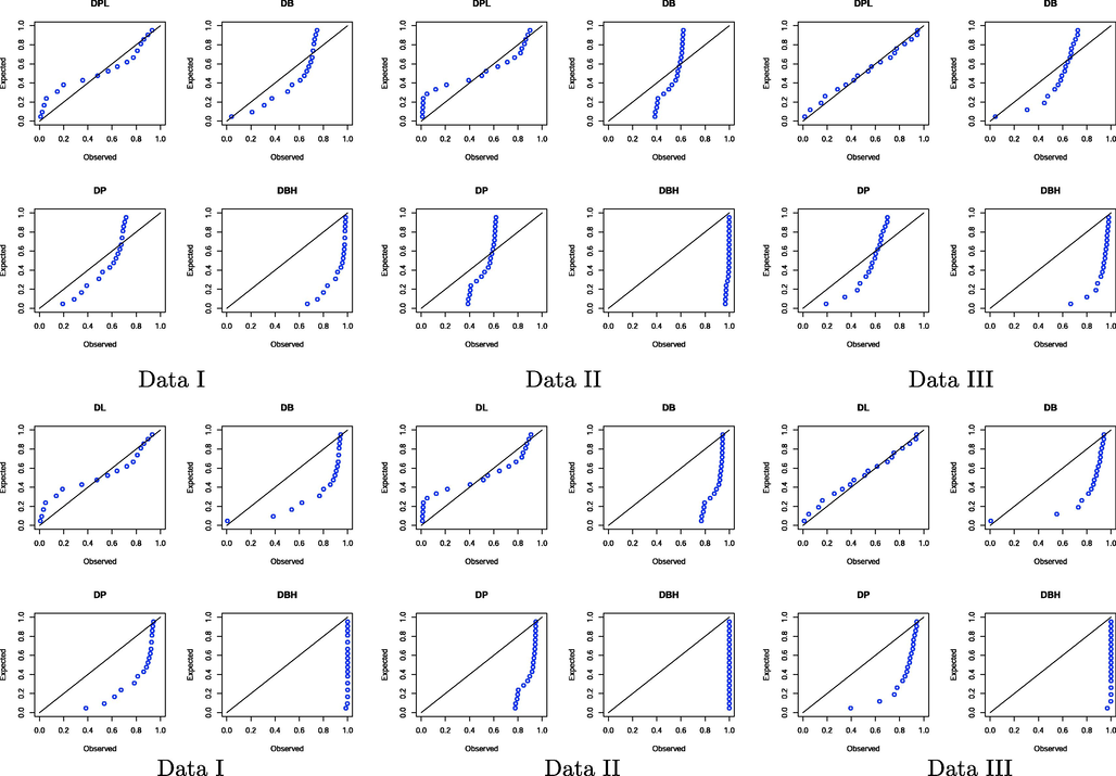
PP plots of the DPL (top panel) and DP (bottom panel) models and other models for three data sets.
Based on the KS and KS-PV, we conclude that the DPL and DL distributions provide adequate fit for the three data sets as compared with other discrete models.
6 Concluding remarks
In this paper, we derive two risk measures called value at risk and tail value at risk for the discrete Poisson-Lindley (DPL) and discrete Lindley (DL) distributions, and study their behavior using numerical simulations. Further, we discuss the estimation of the parameters for the two discrete distributions using five classical methods of estimation namely, the maximum likelihood, least squares, weighted least squares, percentiles, and Cramér-von Mises. We present detailed simulation results to compare these estimators in terms of mean square errors, average absolute biases, mean relative estimates, and total absolute relative errors of the parameters. The simulation study illustrates that all classical estimators perform very well and their performance ordering, depending on overall ranks, from best to worst is WLSE, LSE, PCE, CVME, and MLE for the DPL distribution. Further, the performance ordering for the DL parameter is PCE, WLSE, LSE, CVME, and MLE. The practical importance of the two distributions is discussed using three real-life data sets form medicine field. The DPL and DL distributions provide better fit for the three analyzed data than some other discrete distributions.
Funding
This project is supported by Researchers Supporting Project number (RSP-2020/156) King Saud University, Riyadh, Saudi Arabia.
Acknowledgement
The authors would like to thank the Editor and two reviewers for their constructive comments that greatly improved the final version of the manuscript. This work was supported by King Saud University (KSU). The first author, therefore, gratefully acknowledges the KSU for technical and financial support.
Declaration of Competing Interest
The authors declare that they have no known competing financial interests or personal relationships that could have appeared to influence the work reported in this paper.
References
- A new three-parameter exponential distribution with variable shapes for the hazard rate: Estimation and applications. Mathematics. 2020;8(1):135.
- [Google Scholar]
- The heavy-tailed exponential distribution: Risk measures, estimation, and application to actuarial data. Mathematics. 2020;8(8):1276.
- [Google Scholar]
- A new discrete analog of the continuous lindley distribution, with reliability applications. Entropy. 2020;22(6):603.
- [Google Scholar]
- The odd exponentiated half-logistic exponential distribution: estimation methods and application to engineering data. Mathematics. 2020;8(10):1684.
- [Google Scholar]
- A new extended two-parameter distribution: Properties, estimation methods, and applications in medicine and geology. Mathematics. 2020;8(9):1578.
- [Google Scholar]
- Application of coherent risk measures to capital requirements in insurance. North Am. Actuarial J.. 1999;3(2):11-25.
- [Google Scholar]
- Two parameter exponentiated gumbel distribution: Properties and estimation with flood data example. J. Stat. Manage. Syst.. 2017;20(2):197-233.
- [Google Scholar]
- Discrete Burr-Hatke distribution with properties, estimation methods and regression model. IEEE Access. 2020;8:74359-74370.
- [Google Scholar]
- Estimation methods for the discrete Poisson-Lindley distribution. J. Stat. Comput. Simul.. 2009;79(1):1-9.
- [Google Scholar]
- Computer methods for estimating Weibull parameters in reliability studies. IRE Trans. Reliab. Quality Control 1958:15-22.
- [Google Scholar]
- A graphical estimation of mixed Weibull parameters in life-testing of electron tubes. Technometrics. 1959;1(4):389-407.
- [Google Scholar]
- Loss models: from data to decisions,. Vol vol. 715. John Wiley & Sons; 2012.
- Discrete Burr and discrete Pareto distributions. Stat. Methodol.. 2009;6(2):177-188.
- [Google Scholar]
- Statistical models and methods for lifetime data. Vol vol. 362. John Wiley & Sons; 2011.
- Fitting the generalized Pareto distribution to data using maximum goodness-of-fit estimators. Comput. Stat. Data Anal.. 2006;51(2):904-917.
- [Google Scholar]
- Comments and queries comment on ’an estimation procedure for mixtures of distributions’ by Choi and Bulgren. J. Roy. Stat. Soc.: Ser. B (Methodol.). 1971;33(2):326-329.
- [Google Scholar]
- A new generalization of the exponentiated pareto distribution with an application. Am. J. Math. Manage. Sci.. 2018;37(3):217-242.
- [Google Scholar]
- Estimation methods of alpha power exponential distribution with applications to engineering and medical data. Pakistan J. Stat. Oper. Res. 2020:149-166.
- [Google Scholar]
- Poisson exponential distribution: different methods of estimation. J. Appl. Stat.. 2018;45(1):128-144.
- [Google Scholar]
- On the generalized extended exponential-weibull distribution: Properties and different methods of estimation. Int. J. Computer Math.. 2020;97(5):1029-1057.
- [Google Scholar]
- Least-squares estimation of distribution functions in Johnson’s translation system. J. Stat. Comput. Simul.. 1988;29(4):271-297.
- [Google Scholar]


