Translate this page into:
The Marshall-Olkin length-biased exponential distribution and its applications
⁎Corresponding author. ahsanshani36@gmail.com (Muhammad Ahsan ul Haq)
-
Received: ,
Accepted: ,
This article was originally published by Elsevier and was migrated to Scientific Scholar after the change of Publisher.
Peer review under responsibility of King Saud University.
Abstract
A generalization of the length-biased exponential distribution called the Marshall-Olkin length-biased exponential distribution is proposed in the present paper. Statistical properties of the proposed model are discussed. The parameters of the proposed model are estimated by maximum likelihood estimation method. The performance of the maximum likelihood estimates is investigated by means of a Monte Carlo simulation study. The appropriateness of the model is validated empirically by utilizing a real life data set.
Keywords
Length-biased exponential
Marshall-Olkin
Order statistic
Rényi entropy
1 Introduction
Most of the statistical analyses deal with real life data sets under appropriate selection of models. The model selection is also an important issue for reliable estimation of the model parameters. Recently, some generalizations of the exponential distribution are proposed for modeling lifetime data due to some interesting properties such as “lack of memory” (Ristić and Kundu, 2015).
Many generalizations of the exponential distribution are developed in recent years such as the exponentiated exponential (Gupta and Kundu, 1999, 2001), generalized exponentiated moment exponential (Iqbal et al., 2014), extended exponentiated exponential (Abu-Youssef et al., 2015), Marshall-Olkin exponential Weibull (Pogány et al., 2015), Marshall-Olkin generalized exponential (Ristic and Kundu, 2015), and exponentiated moment exponential (Hasnain et al., 2015) distributions.
In the rest of the paper, we define the new model in Section 2, the statistical properties of the proposed distribution are discussed in Section 3, and estimation of parameters by using maximum likelihood estimation method is presented in Section 4. A simulation study and an application of proposed model on real life data set are provided in Section 5. In Section 6, concluding remarks are presented.
2 The new model
The weighted or moment distributions arise in the context of unequal probability sampling; have a great importance in reliability, biomedicine, and ecology, among others.
Dara and Ahmad (2012) proposed the moment exponential distribution (here we will call it Length-Biased Exponential (LBE) distribution) through assigning weight to the exponential distribution by following the idea of Fisher (1934). Dara and Ahmad (2012) proved that the LBE is more flexible than the exponential distribution.
The Probability Density Function (PDF) and Cumulative Distribution Function (CDF) of LBE distribution are;
The procedure of adding one or two shape parameters to a family of distributions for getting more flexibility is a well-known technique in the literature. Marshall and Olkin (1997) proposed a simple method of adding a shape parameter into a family of distributions. Considering a baseline CDF,
, of a random variable
, then the CDF of the Marshall and Olkin-G (MO-G) family of distributions is
The corresponding PDF (3) is given by
The major motivation of the MO family is given as follows: Let where are a sequence of IID random variables from and is a random variable with probability mass function . Then, the CDF of is defined by; which is equivalent to (3).
Several authors used the MO-G family to extend well-known distributions in the last few years for getting more flexible models. For example, the extended Weibull distribution (Marshall and Olkin, 1997), MO Weibull (Ghitany et al., 2005), MO Pareto (Ghitany, 2005), MO gamma (Ristic et al., 2007), MO Lomax (Ghitany et al., 2007), MO linear failure-rate (Ghitany and Kotz, 2007), MO log-logistic (Gui, 2013), MO Frechet (Krishna et al., 2013) and MO exponential Weibull (Pogány et al., 2015) distributions.
In this article, we proposed a new extension of the LBE distribution called the Marshall Olkin Length-Biased Exponential (MOLBE) distribution. In fact, the new model is constructed using the MO family of distributions. A comprehensive description of some of its mathematical properties with the hope that it will attract wider applications in reliability, engineering and other areas of research is provided. It is justified that the MOLBE distribution can provide good fits for a real life data set.
The new distribution can be defined by inserting Eq. (2) in Eq. (3). Then, the CDF of the MOLBE model, say
is;
By putting Eqs. (1) and (2) in Eq. (4), we obtain the PDF of the MOLBE distribution
For , the MOLBE reduces to the LBE distribution.
The Survival Function (SF) and the Hazard Rate Function (HRF) of X are; and
By using the following generalized binomial expansion and the power series (for),
Ay useful linear representation for the PDF of Eq. (6) is;
A simple motivation of the MOLBE distribution follows by considering a parallel system with independent components and suppose that a random variable has the geometric distribution with the probability mass function and. Let represent the lifetimes of each component and suppose that they have the LBE distribution given in (1). Then a random variable represents the lifetime of the system. Therefore, the random variable follows the MOLBE in (5).
Figs. 1 and 2 show some possible shapes of the PDF, and HRF of the MOLBE distribution for selected values of parameters.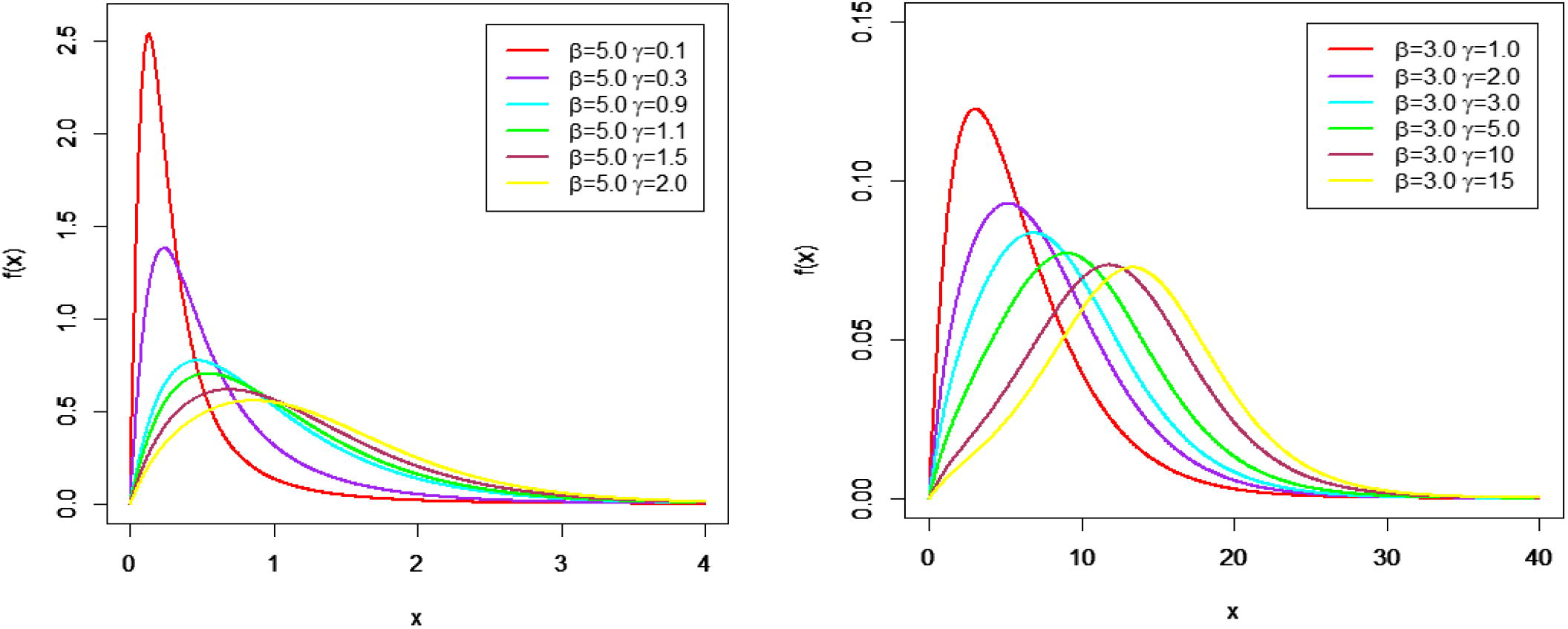
Graph for MO-ME density function at different parameter values.
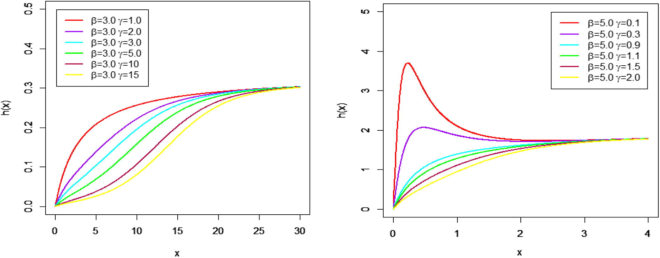
Graph for hazard rate function at different parameter values.
Fig. 1 shows the unimodal behavior for the density of the MOLBE distribution with various choices of parameters. Fig. 2 shows that the HRF of the MOLBE model can be increasing or unimodal.
3 Mathematical properties
In this section, some fundamental properties of MOLBE distribution including moments, generating function, incomplete moments, entropies, mean residual life and mean inactivity time are presented.
3.1 Moments
The th moment of is defined by;
Using (7), we can write
After some algebra, we have
The moment generating function of is defined by
Thus, we have
The effects of the parameters on the mean, variance, skewness and kurtosis are displayed in Figs. 3 and 4, respectively.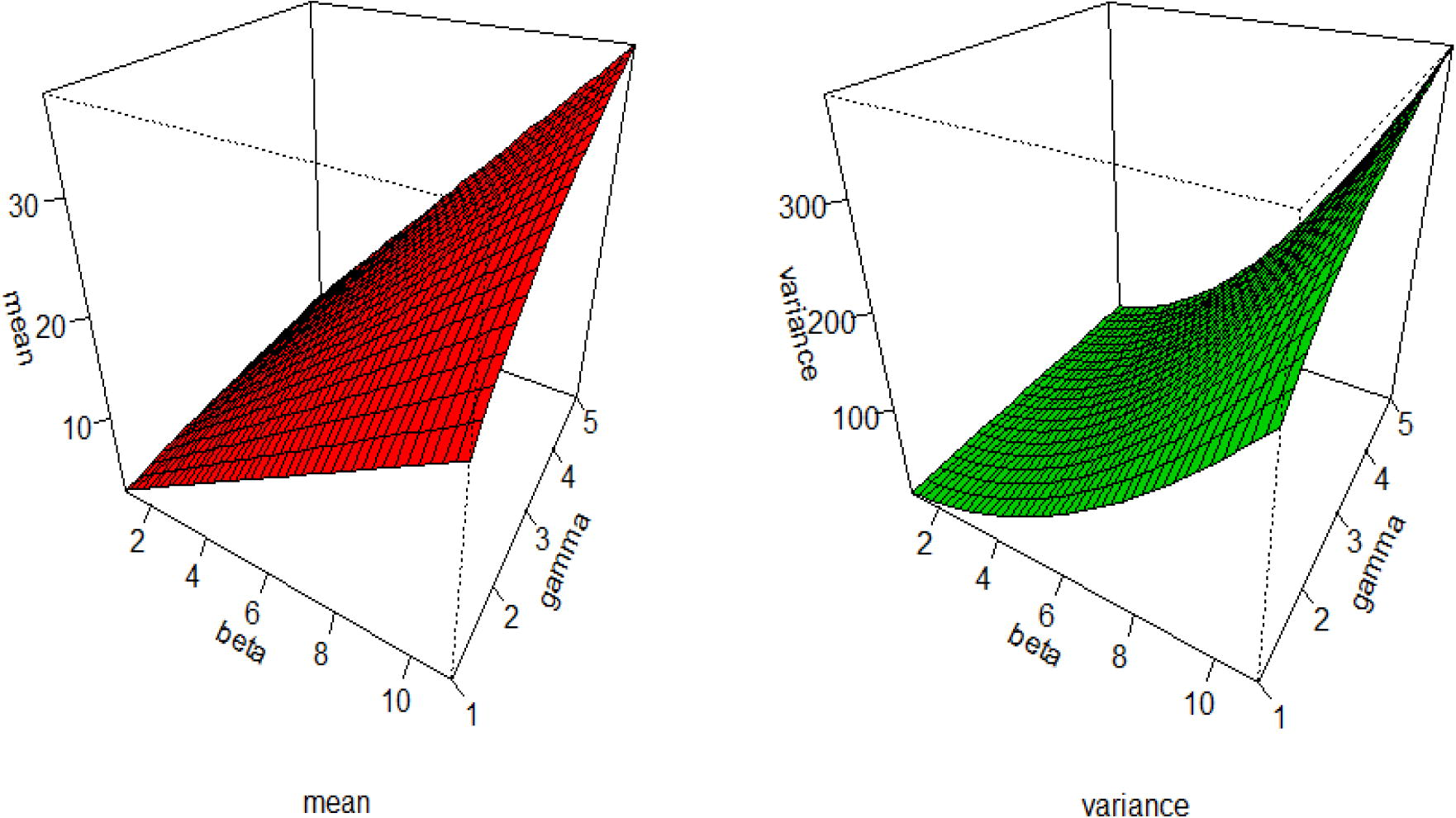
Plots of the mean and variance for the MOLBE distribution.
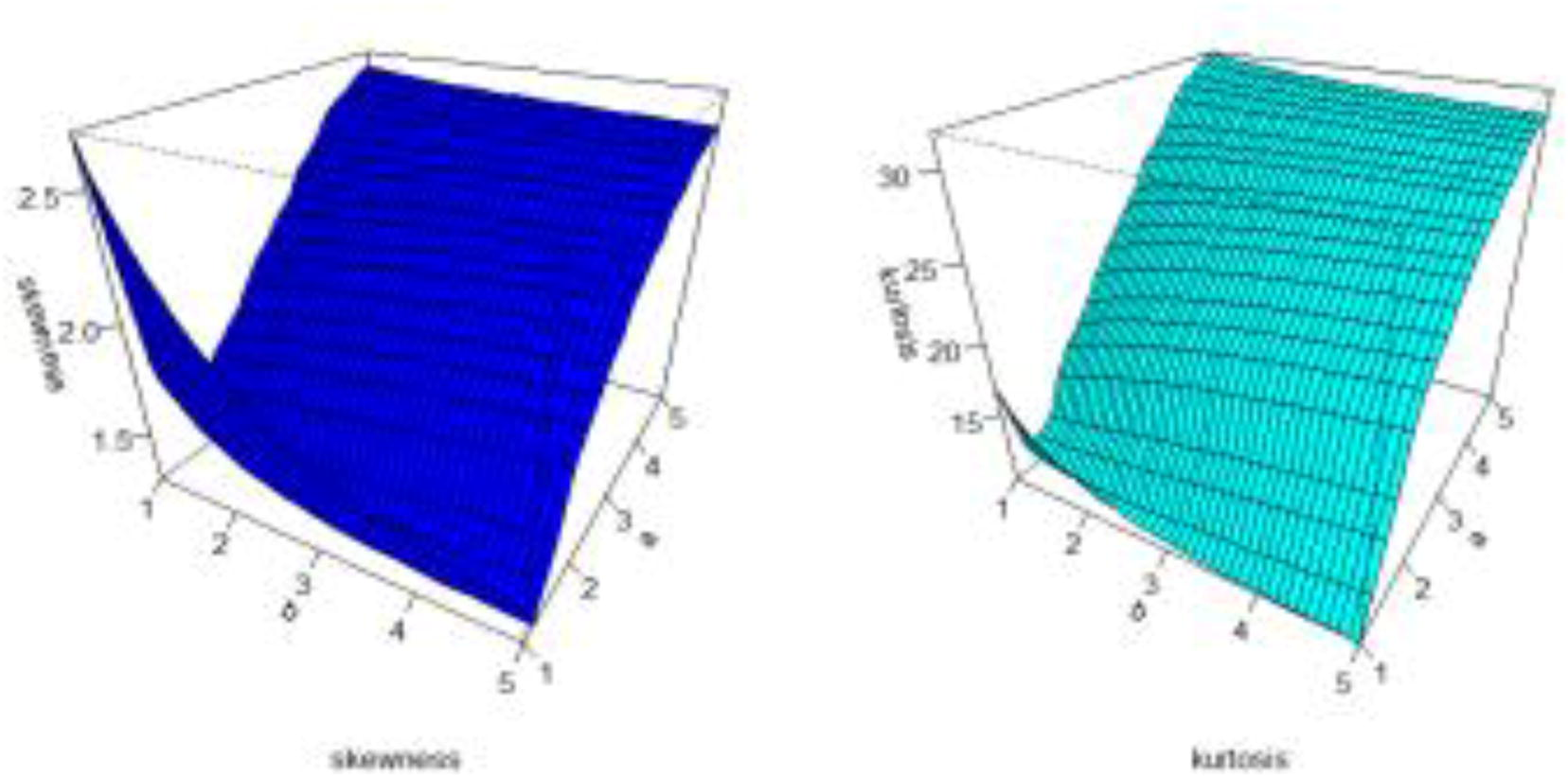
Plots of the skewness and kurtosis for the MOLBE distribution.
The rth incomplete moment of is defined by
Based on Eq. (7), we obtain
Then, the rth incomplete moment of
reduces to
3.2 Entropies
The Rényi entropy of a random variable represents a measure of variation of the uncertainty and it is defined (for ) as;
where
Using Eq. (6), we have
After some simplifications, we obtain
Then, we can write
The q-entropy, , is defined by
Using , we obtain
3.3 Mean residual life and mean inactivity time
The Mean Residual Life (MRL) (or the life expectancy at age ) represents the expected additional life length for a unit, which is alive at age . It has many applications in biomedical sciences, life insurance, maintenance and product quality control, economics and social s tudies, demography and product technology.
The MRL is defined as;
where is first incomplete moment of follows from (8) with
Substituting in Eq. in (9), we can write
The Mean Inactivity Time (MIT) represents the waiting time elapsed since the failure of an item on condition that this failure had occurred in ( ).
The MIT of is given ( ) by
By inserting in the last equation, the MIT of comes out as;
4 Estimation
In this section, the unknown parameters of the MOLBE distribution are estimated by using the maximum likelihood method. Let be a random sample of size from the MOLBE distribution and let be the vector of parameters. The likelihood function for the MOLBE distribution is;
The log-likelihood function, reduces to
The score vector components, , are given by
and
The complicated system of nonlinear equations obtained from can be solved using numerical Newton–Raphson type methods. However, it is much simpler to maximize the log-likelihood function directly by means of the R (optim function), SAS (PROC NLMIXED), Mathcad or Ox program (sub-routine MaxBFGS).
5 Data analysis
In this section, some simulation results are provided to observe the behavior of the MLEs in terms of the sample size . The importance of the MOLBE distribution using real data is also illustrated.
5.1 Simulation study
A small Monte Carlo simulation study is conducted to observe the finite sample behavior of the MLEs of and. All results are obtained from 10,000 Monte Carlo replications and the simulations are carried out using the statistical software R. In each replication, a random sample of size
is generated from the MOLBE(
) distribution. Table 1 lists the means of the MLEs of the MOLBE parameters, biases and the corresponding Mean Squared Errors (MSEs) for sample sizes
,
and
.
Sample size (n)
Parameters
Mean
Bias
MSE
3
0.75
50
3.037
1.0210.037
0.2711.305
0.584
150
3.009
0.8690.009
0.1190.446
0.185
300
3.0002
0.7840.0002
0.0340.120
0.045
3
1.25
50
2.999
1.637−0.001
0.3870.628
1.230
150
3.009
1.3540.009
0.1040.171
0.238
300
3.003
1.2980.003
0.0480.086
0.106
3
2
50
3.001
2.5740.001
0.5740.407
3.031
150
2.990
2.185−0.009
0.1850.129
0.599
300
2.996
2.105−0.004
0.1050.062
0.263
1.5
2
50
1.491
2.600−0.009
0.6000.100
2.997
150
1.494
2.203−0.006
0.2030.031
0.606
300
1.495
2.110−0.004
0.1100.015
0.267
1.5
3
50
1.478
3.913−0.022
0.9130.075
7.157
150
1.480
3.310−0.019
0.3100.023
1.302
300
1.484
3.172−0.016
0.1730.012
0.554
The results in Table 1 reveal that the estimates are stable and quite close to the true parameter values for these sample sizes. Furthermore, as the sample size increases the MSEs decreases in all cases.
5.2 Application
In this section, the importance and flexibility of the new distribution is illustrated by using a real life data set. The data represent the tensile strength of 100 carbon fibers (Flaih et al., 2012). The data are: 3.7, 3.11, 4.42, 3.28, 3.75, 2.96, 3.39, 3.31, 3.15, 2.81, 1.41, 2.76, 3.19, 1.59, 2.17, 3.51, 0.84, 1.61, 1.57, 1.89, 2.74, 3.27, 2.41, 3.09, 2.43, 2.53, 2.81, 3.31, 2.35, 2.77, 2.68, 4.91, 1.57, 2.00, 1.17, 2.17, 0.39, 2.79, 1.08, 2.88, 2.73, 2.87, 3.19, 1.87, 2.95, 2.67, 4.20, 2.85, 2.55, 2.17, 2.97, 3.68, 0.81, 1.22, 5.08, 1.69, 3.68, 4.70, 2.03, 2.82, 2.50, 1.47, 3.22, 3.15, 2.97, 2.93, 3.33, 2.56, 2.59, 2.83, 1.36, 1.84, 5.56, 1.12, 2.48, 1.25, 2.48, 2.03, 1.61, 2.05, 3.60, 3.11, 1.69, 4.90, 3.39, 3.22, 2.55, 3.56, 2.38, 1.92, 0.98, 1.59, 1.73, 1.71, 1.18, 4.38, 0.85, 1.80, 2.12, 3.65.
We shall compare the fits of the MOLBE model with other seven models namely:
-
The Exponential (E) distribution (Nadarajah and Kotz, 2006) with CDF given by
-
The Marshall-Olkin extended exponential (MOEE) distribution (Srivastava et al., 2011) with CDF given by
-
The Exponentiated Exponential (EE) distribution (Gupta and Kundu, 2001) with CDF given by
-
Moment Exponential (ME) distribution (Dara and Ahmad, 2012) with CDF given by
-
Exponentiated Moment exponential (EME) (Hasnain et al., 2015) with CDF given by
The fitted models are assessed based on some goodness-of-fit statistics named: the Akaike Information Criterion (AIC), Bayesian Information Criterion (BIC), Cramér-von Mises (W), Anderson–Darling (AD) and the maximized log-likelihood ( ).
Tables 2 and 3 provide the MLEs of the model parameters and goodness-of-fit measures, respectively. Fig. 5 shows the fitted densities and estimated CDF of the MOLBE distribution.
Distribution
Estimated Parameters
MOLBE
–
23.77
0.515922
E
–
–
0.382936
BE
5.99635
191.696
0.0118252
MOEE
–
77.7225
1.69322
EE
7.878
–
1.021
ME
–
–
1.3057
EME
3.51349
–
0.775339
Distribution
AIC
BIC
A
W
MOLBE
285.956
291.166
−140.978
1.09176
0.21034
E
393.977
396.582
−195.989
17.5557
3.48081
BE
291.056
298.871
−142.528
0.77823
0.15443
MOEE
286.720
291.930
−141.360
0.39549
0.06058
EE
294.910
300.120
−145.455
1.25447
0.23611
ME
333.857
336.462
−165.928
8.14797
1.45650
EME
292.749
297.959
−144.374
1.09176
0.21035
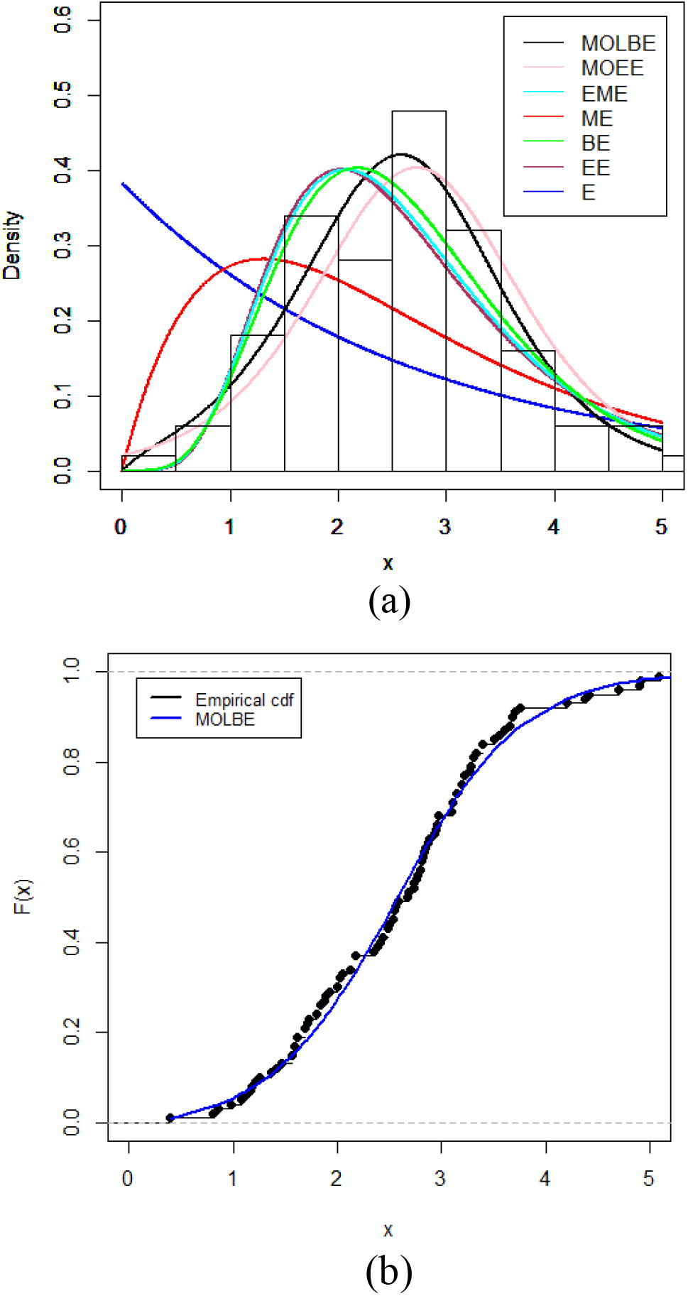
(a) Fitted densities of the MOLBE distribution and other competitive models. (b) Estimated cdf of the MOLBE model and the empirical cdf for the data.
It is clear, from the figures in Table 3 and the plots in Fig. 5, that the MOLBE and MOEE distributions provide good fits to these data. Thus, the MOLBE and MOEE distributions are potential competitors.
6 Conclusions
In this paper, the two-parameter Marshall-Olkin length-biased exponential (MOLBE) distribution is proposed which extends the length-biased exponential (LBE) distribution pioneered by Dara and Ahmad (2012). The mathematical properties of the MOLBE distribution are derived including ordinary and incomplete moments, generating function, entropies, mean residual life and mean inactivity time. The estimation of the model parameters based on MLE are also discussed. The proposed distribution is applied to a real life data set. It provides a better fit than several other competitive models. It is inferred that MOLBE distribution will provide a superior fit to the wider range of applications in statistics.
References
- An extended exponentiated exponential distribution and its properties. Int. J. Comput. Appl.. 2015;121(5)
- [Google Scholar]
- Recent Advances in Moment Distribution and Their Hazard Rates. Lap Lambert Academic Publishing GmbH KG; 2012.
- The effects of methods of ascertainment upon the estimation of frequencies. Ann. Eugenic.. 1934;6:13-25.
- [Google Scholar]
- The exponentiated inverted Weibull distribution. Appl. Math. Inf. Sci. 2012;6(2):167-171.
- [Google Scholar]
- Marshall-Olkin extended Pareto distribution and its application. Int. J. Appl. Math.. 2005;18:17-31.
- [Google Scholar]
- Marshall-Olkin extended Lomax distribution and its applications to censored data. Commun. Statist. Theor. Methods. 2007;36:1855-1866.
- [Google Scholar]
- Marshall-Olkin extended Weibull distribution. And its application to censored data. J. Appl. Statist.. 2005;32:1025-1034.
- [Google Scholar]
- Reliability properties of extended linear failure-rate distributions. Prob. Eng. Inf. Sci.. 2007;21:441-450.
- [Google Scholar]
- Marshall-Olkin extended log- logistic distribution and its application in mimification processes. Appl. Math. Sci.. 2013;7:3396-3947.
- [Google Scholar]
- Theory & methods: generalized exponential distributions. Australian & New Zealand J. Stat.. 1999;41(2):173-188.
- [Google Scholar]
- Exponentiated exponential family: an alternative to gamma and Weibull distributions. Biometrical J.. 2001;43(1):117-130.
- [Google Scholar]
- On exponentiated moment exponential distribution. Pak. J. Statist.. 2015;31(2):267-280.
- [Google Scholar]
- The Marshall-Olkin Fréchet distribution. Commun. Stat. Theory Methods. 2013;42:4091-4107.
- [Google Scholar]
- A new method for adding a parameter to a family of distributions with application to the exponential and Weibull families. Biometrika. 1997;84(3):641-652.
- [Google Scholar]
- The Marshall-Olkin exponential Weibull distribution. Hacettepe J. Math. Stat.. 2015;44:1579-1594.
- [Google Scholar]
- A Marshall-Olkin gamma distribution and minification process. STARS: Stress Anxiety Res. Soc.. 2007;11:107-117.
- [Google Scholar]
- Parameter estimation of Marshall-Olkin extended exponential distribution using markov chain Monte Carlo method for informative set of priors. Int. J. Adv. Sci. Technol.. 2011;2(4):68-92.
- [Google Scholar]


